Zariski-van Kampen Method and Monodromy in Complexified Integrable Systems

Zhiyuan Liu 2200502078@cnu.edu.cn School of Mathematical Science, Capital Normal University

Abstract

We computed the fundamental groups of non-singular sets of some complexified Hamiltonian integrable systems by Zariski-van Kampen method. By our computation, we determined all possible monodromy in complexified planar Kepler problem and spherical pendulum, that is their monodromy groups. We also gave an answer to the conjecture proposed by You and Sun.

Key Words: Complexification; Kepler Problem; Algebraic Curve; Braid Monodromy; Zariski-Van Kampen Method.

AMS Classification Code: 37J35; 37N05; 53D22.

1 Introduction

In a Liouville integrable system $(M,\omega,H,\mu)$ , the famous Liouville-Arnold theorem asserts that the generic fibers of the first integrals $\mu$ are compact Lagrangian tori, these tori are also called angle coordinates, they play an important role in Hamiltonian dynamics and symplectic topology. If the angle coordinates exist globally, that implies geometrically, the symplectic manifold $(M,\omega)$ can be endowed with a global Hamiltonian torus action (the dimension of the torus is half of $M$ ), and the associated moment map $\mu$ coincides with the first integrals $\mu$ . However, in general, such coordinates cannot be constructed globally, because the Lagrangian toric fibrations are not always trivial.

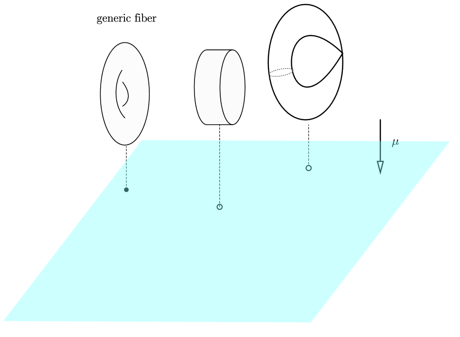
To be specific, suppose $\mu=(F_{1},...,F_{n})$ are $n$ Poisson commuting almost independent first integrals of the Hamiltonian dynamical system $(M,\omega,H)$ (where $H=F_{1}$ ) , let $B\subset\mathbb{R}^{n}$ be the set of regular values such that for each $b\in B$ the fiber $\mu^{-1}(b)$ is generic (the complement of regular values will be called singular set in this paper), then the restriction of $\mu$ gives a toric fibration (see figure 1):

\mu:M^{\prime}\longrightarrow B

where $M^{\prime}$ is the primage of $B$ . The fiber $\mu^{-1}(b)\cong\mathbb{T}^{n}$ is a Lagrangian torus ( $n=\frac{1}{2}\dim M$ ). The action-angle coordinate exists globally if and only if the fibration is trivial.

Refer to caption — Figure 1: Toric fibration determined by Liouville-Arnold theorem

In 1980, Duistmaat developed a notion in [1] called monodromy of a Liouville integrable system, which can perfectly describe the obstructions of the existence of global angle coordinates.

To define the Hamiltonian monodromy, one can consider the period lattice bundle $\Lambda$ over $B$ , where each fiber at $b\in B$ is replaced by the lattice (called period lattice, see [2, §21.2]) $\Lambda_{b}$ of the original torus $\mu^{-1}(b)\cong\mathbb{T}^{n}$ .

Notice that when we restrict the period lattice bundle $\Lambda$ on some loop $\gamma(t)\in\pi_{1}(B,b)$ based at $b\in B$ , we gain a $\mathbb{Z}^{\oplus n}$ -bundle over $\gamma\cong\mathbb{S}^{1}$ , namely

\Lambda|_{\gamma}:=\coprod_{b\in\gamma}\Lambda_{b}\longrightarrow\gamma\cong\mathbb{S}^{1}

The bundle $\Lambda|_{\gamma}$ is determined by a matrix $g(b)\in\mathrm{Aut}(\Lambda_{b})=\mathrm{GL}_{n}(\mathbb{Z})$ , hence it defines a group homomorphism, called the monodromy map:

\mathrm{Mon}:\pi_{1}(B,b)\longrightarrow\mathrm{GL}_{n}(\mathbb{Z}),\,\,\gamma\mapsto g(\gamma(0))

The image of $\mathrm{Mon}$ is called the monodromy group of the integrable system $(M,\omega,H,\mu)$ .

Monodromy is very important in studying Liouville integrable systems. Indeed, Duistmaat showed in [1] that the action-angle coordinate of a system $(M,\omega,H,F_{i})$ exits globally precisely if its monodromy map is trivial (see also [3, p. 393]). After that, various examples of non-trivial monodromy were found, the first such example was the spherical pendulum, found by Cushman in [3] and computed by Duistmaat in [1]. A typical example of a system with trivial monodromy is the Kepler problem, which describes the motion of two bodies under the grivation with one body fixed at the origin. The triviality can be proved by using Pauli and Delauny variables, see [4, 5] for reference. Besides, as was indicated by [6, 7], the monodromy can explain some quantum effects as well.

Some studies in recent decades illustrate that the complexification of some mechanical systems will let us have more benefits. For example, the authors in [8] used the complexification of planar $N-$ body problem proved the finiteness of configurations in planar 5-body problem. The authors in [9] computed the monodromy of complexified spherical pendulum, it has one more rank than the real case. In a recent work [10] of You and Sun, they discovered the non-trivial monodromy phenomenon in complexified planar Kepler problem.

In this paper, we will keep studying the monodromy behavior in complexified planar Kepler problem and spherical pendulum. In particular, we will determine all possible monodromy, that is the monodromy groups of them, by the tools from algebraic geometry and topology. In particular, our computation for complexified planar Kepler problem will give an answer to the conjecture proposed by You and Sun at the end of [10].

In practice, it is difficult to determine all possible monodromy, the main reason is due to the difficulties in computing the fundamental group $\pi_{1}(B,b)$ , especially in the complex settings. In a complexified integrable system, the set $B$ will be the complement of some hypersurfaces in the affine space $\mathbb{C}^{n}$ , and it’s hard to imagine its figure intuitively. Fortunately, in our cases, the regular sets $B$ are both the complement of some affine algebraic curves in $\mathbb{C}^{2}$ , we can compute its fundamental group by tools from algebraic geometry, namely Zariski-van Kampen method, it is a powerful method in studying the topology of algebraic varieties, for example [11, 12].

Our main result is:

Theorem 1.1 (Theorem 3.1 and Theorem 4.1).

$(1)$ . The fundamental group of non-singular set of complexified spherical pendulum is $\mathbb{Z}$ , and its monodromy group is $\mathbb{Z}$ .

$(2)$ . The fundamental group of non-singular set of complexified planar Kepler problem is

\pi_{1}\left(\mathbb{C}^{2}\setminus S\right)=\mathbb{Z}\oplus\mathbb{Z}

Hence consequently, the monodromy group is $\mathbb{Z}_{2}\oplus\mathbb{Z}_{2}$ .

The arrangement of the rest of this paper is as follows:

In section 2, we will introduce the preliminary knowledge in algebraic geometry, including the notion of a holomorphic integrable system. The main tool, that is Zariski-van Kampen method, will be introduced in detail in §2.2. The monodromy of complexified spherical pendulum will be studied in section 3. This is the easier case because all functions are polynomials, hence the complexification is directly. Then in section 4, we will study the complexified planar Kepler problem, the complexification in this case will need a bit modification.

2 Preliminaries

2.1 Complex Integrable System

We first recall that, an Abelian variety $T$ is a compact complex torus $T=\mathbb{C}^{g}/\Lambda$ which can be embedded to some projection space, $\Lambda\cong\mathbb{Z}^{2g}$ is called the lattice of $T$ .

It is well-known that not all compact complex tori admit a projective embedding, it depends on the properties of lattice $\Lambda$ . The conditions on the lattice such that the torus is projective are called Riemann conditions.

Theorem 2.1 (Riemann Conditions, [13]).

A compact complex torus $T=\mathbb{C}^{g}/\Lambda$ is an Abelian variety if and only if $\Lambda$ admits a Riemann form, that is a positive-definite Hermitian form $H$ on $\mathbb{C}^{g}$ such that the image part $\mathrm{Im}\,H(\Lambda,\Lambda)\subset\mathbb{Q}$ .

Now, we can formulate what is a complex integrable system. Let $(M,\omega)$ be a real symplectic manifold of dimension $2n$ , $H$ a Hamiltonian defined on $M$ .

Definition 2.1 (Complex integrable system, [14]).

A real Hamiltonian system $(M,\omega,H)$ is called a complex integrable system, if there exists a complex $2n-$ dimensional holomorphic symplectic manifold $(X,\tau)$ , that is $X$ is a complex manifold together with a symplectic $(2,0)-$ form $\omega$ , and a holomorphic map

\mu=(f_{1},...,f_{n}):X\longrightarrow B\subset\mathbb{C}^{n}

onto a Zariski dense open subset $B$ , such that

$(1)$ . $(M,\omega)$ is the real part of $(X,\tau)$ , and $\omega$ is the restriction of $\tau$ along $\omega$ .

$(2)$ . $\mu$ is submersive and proper.

$(3)$ . $f_{1},...,f_{n}$ are Poisson commuting functions on $(X,\tau)$ .

Remark 2.1.

(1). In algebraic geometry, an algebraic integrable system is just referred to an algebraic symplectic variety, together with $n$ Poisson commuting functions, such that the generic fibers are Lagrangian Abelian varieties. Here, we take the Mumford’s definition because all complex integrable systems that will be considered in this paper are the complexification from the real case. However, the Mumford’s definition implies that the generic fibers are affine parts (or can be extended) to Abelian varieties. For a discussion of some other possible definitions of complex integrable systems, we refer to [15, §5].

(2).Different from the Kähler manifolds (where $\omega$ is a (1,1)-form), holomorphic symplectic manifolds have more special geometry, see [16, 17] for more detail. $\clubsuit$

There are various examples of complex integrable systems. The simplest examples can be constructed from the complexification of some real Liouville integrable systems, and the complexified spherical pendulum and planar Kepler problem are such examples. More interesting example is the Hitchin systems [18], which are defined on the cotangent bundle of the moduli space of Higgs bundles.

2.2 Braid Monodromy and Zariski-van Kampen Method

This section will introduce the necessary tools from algebraic geometry and algebraic topology, namely braid monodromy and Zariski-van Kampen method, which will be used in proving our main results. A good reference in this subject can be found in [19].

2.2.1 Braid Groups

We first introduce what are geometric braids, for more detailed contents on braid groups can be found in [20].

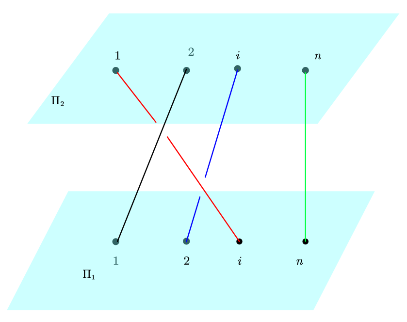
Let $\Pi_{1},\Pi_{2}$ be two parallel planes in $\mathbb{R}^{3}$ , in particular, we assume they both parallel to the $xOy$ -plane, and $\Pi_{2}$ is above $\Pi_{1}$ in the sense that $\Pi_{2}$ has larger $z-$ component. There are $n$ marked ordered positions on each plane $\Pi_{i}$ , namely $1,2,...,n$ , we assume the lines joining the corresponding positions are all vertical to the both planes $\Pi_{i}$ , see figure 2.

Definition 2.2 ([20]).

A geometric braid on $n$ strings is a family of simple arcs $(\beta_{1},\beta_{2},...,\beta_{n})$ in $\mathbb{R}^{3}$ , where each arc $\beta$ is connecting the $i-$ th position in $\pi_{2}$ and the $\sigma(i)-$ th position in $\Pi_{1}$ for some $\sigma\in S_{n}$ , and each two arcs do not intersect.

If all strings in a braid are connecting correspondingly by the order, we call such a braid the identity, denoted by $1$ . Two $n-$ string geometric braid $(\beta_{1},...,\beta_{n})$ and $(\gamma_{1},...,\gamma_{n})$ are called equivalent, if they can be continuously deformed to each other.

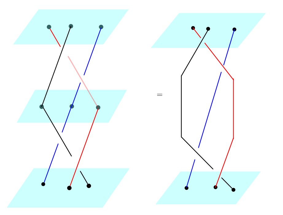
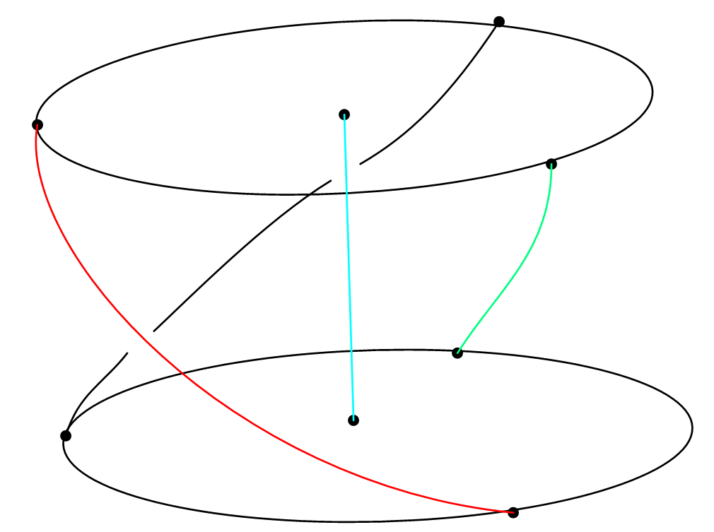
The product or composition of two braids is defined to be the juxtaposition, see figure 3. Clearly, the braids product satisfy the associative law, and any braid product with the identity is itself. Hence the collection of all braids with $n$ strings forms a group, called braid groups, denoted by $B_{n}$ .

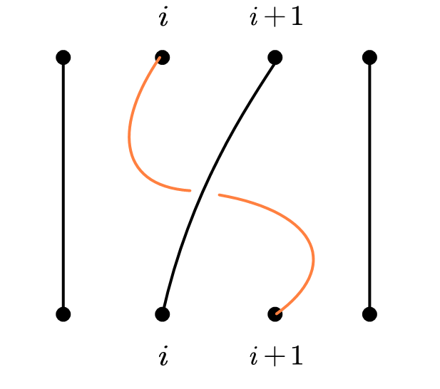
Although braids can be complicated, they can be write as the products of a sequel of simple braids, denoted $\sigma_{i}$ . $\sigma_{i}$ is the braid with just the $i-$ th and the $(i+1)-$ th position interchange and only once, see figure 4. These $\sigma_{i}$ forms the generators in the braid group $B_{n}$ , and the generation is given by [20]

B_{n}=\left\langle\sigma_{1},...,\sigma_{n-1}\left|\begin{cases}\sigma_{i}\sigma_{j}=\sigma_{j}\sigma_{i}&|i-j|\geq 2\\ \sigma_{i}\sigma_{i+1}\sigma_{i}=\sigma_{i+1}\sigma_{i}\sigma_{i+1}&1\leq i\leq n\end{cases}\right\rangle\right.\\

Remark 2.2 (Pure Braids).

If we request every arc $\beta_{i}$ in the $n$ -string braid $(\beta_{1},...,\beta_{n})$ to having same starting-end position, then such a braid will be called the pure braid, the group formed by all pure braids are called pure braid group, denoted by $P_{n}$ , it is clearly that we have the group exact sequence

1\longrightarrow P_{n}\longrightarrow B_{n}\longrightarrow S_{n}\longrightarrow 1

. $\clubsuit$

There are some classical models of braid groups $B_{n}$ which will be needed in this paper.

Example 2.1.

Suppose there are $n$ orderless points moving on the complex plane $\mathbb{C}$ without collisions, the motion of these $n$ points forms a configuration space $X$ , that is

	$\displaystyle X$	$\displaystyle=\left\{(z_{1},...,z_{n})\in\mathbb{C}^{n}\|z_{i}\neq z_{j},i\neq j\right\}/S_{n}$
		$\displaystyle=\left(\mathbb{C}^{n}\setminus\{z_{i}=z_{j},i\neq j\}\right)/S_{n}:=X^{\prime}/S_{n}$

The fundamental group of this configuration space is actually the braid group

\pi_{1}(X,x_{0})\cong B_{n}

In fact, note that the quotient $X^{\prime}\longrightarrow X$ defines an $S_{n}$ -bundle over $X$ , if we choose a section $s$ such that $s(x_{0})=\tilde{x}_{0}\in X^{\prime}$ , then by the homotopy lifting property, each loop in $\pi_{1}(X,x_{0})$ can be lifted to a path in $X^{\prime}$ starting at $\tilde{x}_{0}$ . Notice that every path in $X^{\prime}$ is the motion from one complex plane with ordered positions to the other, and it is in fact an $n$ -string braid illustrated in figure 2, hence $\pi_{1}(X,x_{0})$ is actually the braid group $B_{n}$ . $\clubsuit$

Example 2.2 (Artin representation).

Another interesting model is the mapping class group $\mathcal{M}_{0,1}^{n}$ of the compact Riemann surface with 1 genus, 1 boundary and $n$ marked points, that is the $n-$ punctured disk $\mathbb{D}\setminus\{a_{1},...,a_{n}\}$ , it was proved in [21] that

\mathcal{M}_{0,1}^{n}\cong B_{n}

Mapping class group has its natural action on the fundamental group

\pi_{1}(\mathbb{D}\setminus\{a_{1},...,a_{n}\},a_{0})=\underbrace{\mathbb{Z}*\cdots*\mathbb{Z}}_{n-\text{times}}:=\mathbf{F}_{n}

If we order the generators in $\mathbf{F}_{n}$ in an appropriate way, say $g_{1},...,g_{n}$ , then the action coincides with the Artin representation [21]:

	$\displaystyle\alpha:\mathcal{M}^{n}_{0,1}\cong B_{n}$	$\displaystyle\longrightarrow\mathrm{Aut}\left(\mathbf{F}_{n}\right)$		(1)
	$\displaystyle\alpha(\sigma_{i})(g_{j})$	$\displaystyle=\begin{cases}g_{i+1}&j=i\\ g_{j}g_{i}g_{j}^{-1}&j=i+1\\ g_{j}&\text{otherwise}\end{cases}$		(1)

This model will be used in constructing the braid monodromy. $\clubsuit$

Example 2.3.

Let $\mathbb{C}[y]_{n}$ be the set of monic polynomials with degree $n$ , let $\Delta\subset\mathbb{C}[y]_{n}$ be the subset consisting of polynomials with multiple roots, i.e those monic polynomials $f$ with vanishing discriminants $\Delta_{f}=0$ , then the fundamental group $\pi_{1}(\mathbb{C}[y]_{n}\setminus\Delta)$ is exactly $B_{n}$ .

Indeed, by taking coefficients, the set $\mathbb{C}[y]_{n}\setminus\Delta$ can be identified with the set of $n-$ tuples in $\mathbb{C}^{n}$ with non-zero discriminants, and this is equivalent to the set of $n$ distinct complex roots, it then becomes the model stated in example 2.1, hence its fundamental group is obviously $B_{n}$ . $\clubsuit$

2.2.2 Fundamental Group of the Complement of an Algebraic Curve

Let

f(x,y)=y^{n}+\sum_{i=1}^{n}a_{i}(x)y^{n-1}\in\mathbb{C}[y]_{n}

be a monic degree $n$ polynomial, let $\mathcal{C}$ be the algebraic curve

\left\{(x,y)\in\mathbb{C}^{2}|f(x,y)=0\right\}\subset\mathbb{C}^{2}

We will introduce Zariski-van Kampen method to compute the fundamental group $\pi_{1}(\mathbb{C}^{2}\setminus\mathcal{C})$ .

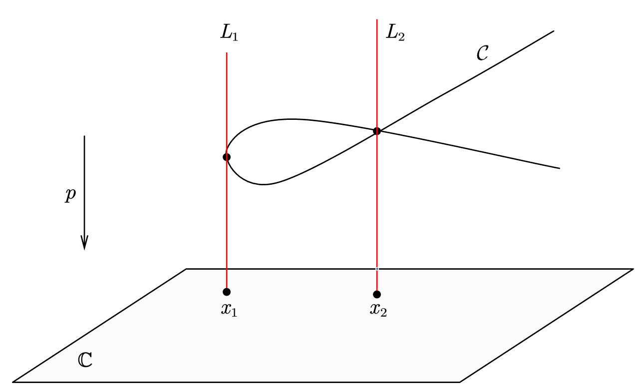
We first define the projection onto the first component

	$\displaystyle p:\mathbb{C}^{2}\setminus\mathcal{C}$	$\displaystyle\longrightarrow\mathbb{C}$
	$\displaystyle(x,y)$	$\displaystyle\mapsto x$

The fiber of the projection is $\mathbb{C}\setminus\{n\,\text{points}\}$ except for those $x$ such that $f(x,y)=f_{x}(y)$ has multiple roots. These points are precisely the branch points of the projection or the singularities of the curve $\mathcal{C}$ . Let $S=\{x_{1},...,x_{s}\}\subset\mathbb{C}$ be the set of all such points. Denoted by $L_{k}=p^{-1}(x_{k})$ , and let

\mathcal{L}=\bigcup_{k=1}^{s}L_{k}

be the union of all such lines, they will be called the singular fibers, see figure 5.

Remark 2.3.

Without loss of generality, we shall assume that all singular fibers $L_{k}$ are in generic position. That is every $L_{k}$ intersects transversally with the curve $\mathcal{C}$ , and cannot contain other singularities or branch points. If some $L_{k}$ is not generic, we can change of the variables on $\mathcal{C}$ so that the projection onto the first component in the new coordinates has the generic singular fibers.

Proposition 2.1 ([11]).

The restriction of the projection $p$ :

p:\mathbb{C}^{2}\setminus(\mathcal{C}\cup\mathcal{L})\longrightarrow\mathbb{C}\setminus S

is a fibration with fiber $F=\mathbb{C}\setminus\{n\,\text{points}\}$ . The structure group of this fiber bundle is precisely the braid group $B_{n}$ .

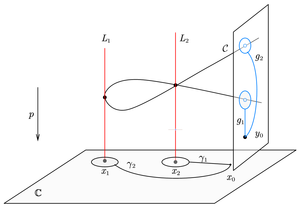
Choose a base point $x_{0}\in\mathbb{C}\setminus S$ and $y_{0}\in F$ , the fundamental groups of the base manifold and the fiber are simply:

\pi_{1}(\mathbb{C}\setminus S,x_{0})\cong\mathbf{F}_{s},\,\pi_{1}\left(F,y_{0}\right)\cong\mathbf{F}_{n}

The fundamental group of the base manifold has an action on the fundamental group of the fiber, this action is called braid monodromy, denoted by $\rho$ :

\rho:\mathbf{F}_{s}\longrightarrow\mathrm{Aut}\left(\mathbf{F}_{n}\right)

The construction of the braid monodromy $\rho$ is as follows.

We take the algebraic curve $f(x,y)=0$ as a map:

	$\displaystyle f:\mathbb{C}$	$\displaystyle\longrightarrow\mathbb{C}[y]_{n}\cong\mathbb{C}^{n}$
	$\displaystyle x$	$\displaystyle\mapsto f_{x}(y)=f(x,y)$

Let $\Delta$ be the subset containing the polynomials with vanishing discriminants (see example 2.3), observe that $f^{-1}(\Delta)$ is precisely $S$ , hence the restriction of $f$ on $\mathbb{C}\setminus S$ induces a homomorphism of fundamental groups:

The braid monodromy is given by the composition of Artin representation $\alpha$ (see example 2.2) and $f_{*}$

\rho=\alpha\circ f_{*}:\mathbf{F}_{s}\longrightarrow\mathrm{Aut}\left(\mathbf{F}_{n}\right)

Hence now, we can apply homotopy exact sequence of fibration:

If we denoted by $\gamma_{1},...,\gamma_{s}$ , $g_{1},...,g_{s}$ the generators of the fundamental groups $\pi_{1}(\mathbb{C}\setminus S,x_{0})$ and $\pi_{1}(F,y_{0})$ respectively, see figure 6, then we can state Zariski-van Kampen method as follows:

Theorem 2.2 (Zariski-van Kampen, [19]).

The fundamental group of total space is the semi-product along braid monodromy:

\pi_{1}\left(\mathbb{C}^{2}\setminus(\mathcal{C}\cup\mathcal{L})\right)\cong\mathbf{F}_{s}\rtimes_{\rho}\mathbf{F}_{n}

In particular, it has the presentation

\pi_{1}\left(\mathbb{C}^{2}\setminus(\mathcal{C}\cup\mathcal{L})\right)=\left\langle\gamma_{1},...,\gamma_{s},g_{1},...,g_{n}|\gamma_{k}^{-1}g_{i}\gamma_{k}=\rho(\gamma_{k})(g_{i})\right\rangle

Moreover, the fundamental group of $\mathbb{C}^{2}\setminus\mathcal{C}$ is the quotient by the normal closure generated by $\gamma_{1},...,\gamma_{s}$ , and it has the presentation

\pi_{1}(\mathbb{C}^{2}\setminus\mathcal{C})=\langle g_{1},...,g_{n}|g_{i}=\rho(\gamma_{k})(g_{i})\rangle

Example 2.4 (The Riemann surface of $\sqrt{z}$ ).

As a simple example, let’s consider the fundamental group of the complement of the curve $X_{\sqrt{z}}:y^{2}=x$ , which is the Riemann surface of the square root function.

Observe that the curve $X_{\sqrt{z}}$ has only one branched point $(0,0)$ in projecting onto the first component, hence $\pi_{1}(\mathbb{C}\setminus S)\cong\mathbb{Z}$ , and braid monodromy will be given in $B_{2}$ . Now choose $\gamma(t)=e^{2\pi\sqrt{-1}}t$ be the generator in $\pi_{1}(\mathbb{C}\setminus S)$ , observe that the change of $y$ is simply $\pm e^{\pi\sqrt{-1}t}$ , hence it yields the braid as $\sigma_{1}$ , by (1), the generators $g_{1},g_{2}$ on the fiber should satisfy the relation $g_{1}=g_{2}$ , hence

\pi_{1}\left(\mathbb{C}^{2}\setminus X_{\sqrt{z}}\right)\cong\mathbb{Z}

$\clubsuit$

More generally, we have

Theorem 2.3 ([19]).

For any irreducible smooth affine algebraic curve $\mathcal{C}$ in $\mathbb{C}^{2}$ , the fundamental group

\pi_{1}\left(\mathbb{C}^{2}\setminus\mathcal{C}\right)\cong\mathbb{Z}

$proof.$ We assume the curve $\mathcal{C}$ has degree $d$ . Since it is irreducible and smooth, the projection onto the first component will only have branch points with branching order $d$ . Therefore, near each branch point, the curve has the local expression $y^{d}=x$ , that gives a braid as $\sigma_{1}\sigma_{2}\cdots\sigma_{d-1}\in B_{d}$ . Therefore, by Zariski-van Kampen method, we can compute the generators $g_{1},...,g_{d}$ of $\pi_{1}\left(\mathbb{C}^{2}\setminus\mathcal{C}\right)$ by

g_{i}=\sigma_{1}\cdots\sigma_{d-1}(g_{i})\Rightarrow g_{1}=g_{2}=\cdots=g_{d}

hence the fundamental group is $\mathbb{Z}$ , as was to be shown. $\clubsuit$

More interesting examples can be found in [19].

3 Complexified Spherical Pendulum

3.1 Complexification

The configuration space of spherical pendulum is the unit sphere

\mathbb{S}^{2}=\left\{\left.(x_{1},x_{2},x_{3})\in\mathbb{R}^{3}\right|\sum_{i=1}^{3}x_{i}^{2}=1\right\}

The configuration space is the cotangent bundle $T^{*}\mathbb{C}^{2}$ . If we denote $\langle\cdot,\cdot\rangle$ the Euclidean inner product on $\mathbb{R}^{3}$ , the cotangent bundle can be write as

T^{*}\mathbb{S}^{2}=\{(\mathbf{x},\mathbf{v})\in\mathbb{S}^{2}\times\mathbb{R}^{3}|\langle\mathbf{x},\mathbf{v}\rangle=0\}

The Hamiltonian is

H(\mathbf{x},\mathbf{v})=\frac{1}{2}\|\mathbf{v}\|^{2}+x_{3}:T^{*}\mathbb{S}^{2}\longrightarrow\mathbb{R}

Lie group $\mathrm{SO}(2)$ has a Hamiltonian action on $T^{*}\mathbb{S}^{2}$

	$\displaystyle\mathrm{SO}(2)\times T^{*}\mathbb{S}^{2}$	$\displaystyle\longrightarrow T^{*}\mathbb{S}^{2}$
	$\displaystyle(A,(\mathbf{x},\mathbf{v}))$	$\displaystyle\mapsto(A\mathbf{x},A\mathbf{v})$

with the moment map

J(\mathbf{x},\mathbf{v})=x_{1}v_{2}-x_{2}v_{1}:T^{*}\mathbb{S}^{2}\longrightarrow\mathbb{R}

This moment $J$ is also known as the angular moment. Together with the Hamiltonian $H$ , $\mu=(H,J)$ defines the first integrals of the spherical pendulum, we call $\mu$ the energy-momentum map.

Since everything here is polynomial, we can complexify every directly to a complex integrable system.

Let $\langle\cdot,\cdot\rangle$ be the standard symmetric bilinear form on $\mathbb{C}^{3}$ , the configuration space is now a complexified sphere:

\mathbb{CS}^{2}=\left\{\mathbf{x}\in\mathbb{C}^{3}|\langle\mathbf{x},\mathbf{x}\rangle=1\right\}

and the phase space is simply

T^{*}\mathbb{CS}^{2}=\{(\mathbf{x},\mathbf{v})\in\mathbb{S}^{2}\times\mathbb{C}^{3}|\langle\mathbf{x},\mathbf{v}\rangle=0\}\subset\mathbb{C}^{3}\times\mathbb{C}^{3}

It is now a holomorphic symplectic manifold, in particular, it is an affine variety in $\mathbb{C}^{3}\times\mathbb{C}^{3}$ .

The complex Lie group

\mathrm{SO}(2,\mathbb{C})=\left\{\left.A=\begin{pmatrix}a&-b\\ b&a\end{pmatrix}\in\mathrm{GL}_{2}(\mathbb{C})\right|a^{2}+b^{2}=1\right\}\cong\mathbb{C}^{*}

has a natural Hamiltonian action on $T^{*}\mathbb{CS}^{2}$ given by

A\cdot(\mathbf{x},\mathbf{v}):=\left(\begin{pmatrix}A&0\\ 0&1\end{pmatrix}\mathbf{x},\begin{pmatrix}A&0\\ 0&1\end{pmatrix}\mathbf{v}\right)

the moment map, called the complexified angular moment, is given by

J(\mathbf{x},\mathbf{v})=x_{1}v_{2}-x_{2}v_{1}:T^{*}\mathbb{CS}^{2}\longrightarrow\mathbb{C}

The complexified energy-momentum map will still be denoted by $\mu=(H,J)$ . Hence now, the spherical pendulum becomes a complex integrable system in sense of definition 2.1.

3.2 Singular Set and Monodromy

Following [9], we define new coordinates $(w_{1},w_{2},w,z_{1},z_{2},z):=(\mathbf{w},\mathbf{z})$ on $\mathbb{C}^{3}\times\mathbb{C}^{3}$ :

	$\displaystyle w_{1}$	$\displaystyle=x_{1}+\sqrt{-1}x^{2},\,\,w_{2}=x_{1}-\sqrt{-1}x_{2}$
	$\displaystyle z_{1}$	$\displaystyle=v_{1}+\sqrt{-1}v_{2},\,\,z_{2}=v_{1}-\sqrt{-1}v_{2}$

hence the defining equation for $T^{*}\mathbb{CS}^{2}$ is

T^{*}\mathbb{CS}^{2}:\begin{cases}w_{1}w_{2}+w^{2}=0\\ w_{1}z_{2}+w_{2}z_{1}+2wz=0\end{cases}

The energy-momentum map can be re-write under the new coordinates as:

\mu(\mathbf{w},\mathbf{z})=(x,y):=\left(\frac{z_{1}z_{2}+z^{2}}{2}+w,\frac{w_{2}z_{1}-w_{1}z_{2}}{\sqrt{-1}}\right)

Proposition 3.1 ([9]).

Under the notation above, we have

$(1).$ For each $\mathbf{c}=(x,y)\in\mathbb{C}^{2}$ , the fiber $\mu^{-1}(\mathbf{c})$ of the energy-momentum map is a $\mathbb{C}^{*}-$ bundle over the punctured elliptic curve

R_{\mathbf{c}}:=\left\{(w,z)\in\mathbb{C}^{2}|z^{2}=2\left(w^{2}-1\right)(w-x)-y^{2}\right\}\setminus\left\{(\pm 1,0)\right\}

(2)

$(2).$ The singular set such that the energy-moment map $\mu$ has non-generic fibers is the algebraic curve

S=\left\{(x,y)\in\mathbb{C}^{2}\left|\frac{27}{4}y^{4}+2xy^{2}(x^{2}-9)-4(x^{2}-1)^{2}=0\right.\right\}

(3)

proof. (1). Recall that the map

\begin{pmatrix}a&-b\\ b&a\end{pmatrix}\mapsto a+b\sqrt{-1}:=\lambda

gives an isomorphism between $\mathrm{SO}(2,\mathbb{C})$ and $\mathbb{C}^{*}$ , and the Hamiltonian $\mathrm{SO}(2,\mathbb{C})$ action can be reduced to the $\mathbb{C}^{*}$ action by scalar product.

From [9, Proposition 2.1], we know the image of the quotient map

\pi:T^{*}\mathbb{CS}^{2}\longrightarrow T^{*}\mathbb{CS}^{2}/\mathrm{SO}(2,\mathbb{C})

is the affine variety

\left\{(w,z,x,y)\in\mathbb{C}^{4}|z^{2}=2\left(w^{2}-1\right)(w-x)-y^{2}\right\}\setminus\{(\pm 1,0,\pm 1,0)\}

By Noether’s theorem, energy-momentum map $\mu$ is constant on the orbits, hence it can be descent to the quotient space $T^{*}\mathbb{CS}^{2}/\mathrm{SO}(2,\mathbb{C})$ , denoted by $\tilde{\mu}$ . Therefore, $\mu^{-1}(\mathbf{c})$ is an $\mathbb{C}^{*}-$ bundle over $\tilde{\mu}^{-1}(\mathbf{c})$ . Notice that, for each fixed $\mathbf{c}\in\mathbb{C}^{2}$ , the fiber $\tilde{\mu}^{-1}(\mathbf{c})$ is exactly the $R_{\mathbf{c}}$ defined in (2), that proves the claim.

(2). Let $\mathcal{R}$ be the elliptic curve defined in (2), we notice that $\mathcal{R}$ is nonsingular, if and only if the discriminant of

f_{\mathbf{c}}(w)=2\left(w^{2}-1\right)(w-x)-y^{2}

vanishes. Its vanishing locus is precisely formulated by (3). Let $M^{\prime}$ be the primage of $\mathbb{C}^{2}\setminus S$ under $\mu$ , to obtain the desired conclusion, we also need to show

\mu:M^{\prime}\longrightarrow\mathbb{C}^{2}\setminus S

has maximal rank everywhere, it follows from [9, Proposition 2.2]. $\clubsuit$

Theorem 3.1.

The fundamental group of the non-singular set $\mathbb{C}^{2}\setminus S$ is $\mathbb{Z}$ , and the monodromy group of complex spherical pendulum is $\mathbb{Z}$

$proof$ . We notice that the defining equation (3) for $S$ is smooth and irreducible, hence by theorem 2.3 we have

\pi_{1}\left(\mathbb{C}^{2}\setminus S\right)\cong\mathbb{Z}

Denoted by $\Gamma$ a generator of the fundamental group.

To compute the monodromy group, we define the period lattice in the following way.

Fix a $\mathbf{c}=(x,y)\in\mathbb{c}^{2}\setminus S$ , first give $M_{\mathbf{c}}=\mu^{-1}(\mathbf{c})$ a partial compactification $\overline{M}_{\mathbf{c}}$ by compactifying the elliptic curve $\mathcal{R}$ defined in (2), let $\overline{R}_{\mathbf{c}}$ be the compactification of $R_{\mathbf{c}}$ . Then we will need following results:

Lemma 3.1 ([9]).

$(1)$ . The forms

\omega_{1}=\frac{dw}{z},\,\,\omega_{2}=\sqrt{-1}\frac{wz-\sqrt{-1}y}{z(w^{2}-1)}dw-\frac{dw_{1}}{w_{1}}

can be analytically continued to $\overline{M}_{\mathbf{c}}$ .

$(2)$ . The following set

\Lambda_{\mathbf{c}}:=\left\{\left.\left(\int_{\gamma}\omega_{1},\int_{\gamma}\omega_{2}\right)\right|\gamma\in H_{1}\left(\overline{M}_{\mathbf{c}};\mathbb{Z}\right)\right\}

(4)

is a lattice in $\mathbb{C}^{2}$ , its $\mathbb{Z}-$ rank is $3$ , the generating vectors are

(\lambda_{1},\mu_{1}),\,(\lambda_{2},\mu_{2}),\,(0,2\pi)

where

\lambda_{i}=\int_{\gamma_{i}}\frac{dw}{z},\,\,\mu_{i}=\sqrt{-1}\int_{\gamma_{i}}\frac{wz-\sqrt{-1}y}{z(w^{2}-1)}dw

here $\gamma_{i}$ ’s are the generators of $H_{1}(\overline{R}_{\mathbf{c}};\mathbb{C})\cong\mathbb{Z}\oplus\mathbb{Z}$ .

$(3)$ . The Hamiltonian monodromy matrix of the lattice $\Lambda_{\mathbf{c}}$ along $\Gamma$ is

\mathrm{Mon}(\Gamma)=\begin{pmatrix}1&-1&0\\ 0&1&0\\ 0&0&1\end{pmatrix}

Then our conclusion follows directly from lemma 3.1. For a detailed proof of lemma 3.1 can be found in [9, §4 and §6]. $\clubsuit$

For more interesting computations of Hamiltonian monodromy of spherical pendulum, we refer to [22].

Remark 3.1.

The lattice $\Lambda_{\mathbf{c}}$ defined in (4) comes from the generalised Abel-Jacobi map $\mathcal{AJ}$ [23], which is defined as

	$\displaystyle\mathcal{AJ}:\overline{M}_{\mathbf{c}}$	$\displaystyle\longrightarrow\mathbb{C}^{2}$
	$\displaystyle p$	$\displaystyle\mapsto\left(\int_{p_{0}}^{p}\omega_{1},\int_{p_{0}}^{p}\omega_{2}\right)$

where $p_{0}$ is a fixed point in $\overline{M}_{\mathbf{c}}$ . It was shown in [9, Theorem 5.1] that the Abel-Jacobi map $\mathcal{AJ}$ has a globally defined inverse. $\clubsuit$

4 Complexified Planar Kepler Problem

Let’s first recall the data in the usual planar Kepler problem, more detailed contents can be found in [4, 5].

The phase space is the symplectic manifold $T^{*}(\mathbb{R}^{2}\setminus\{\mathbf{0}\})\cong(\mathbb{R}^{2}\setminus\{\mathbf{0}\})\times\mathbb{R}^{2}$ endowed with the standard symplectic form:

\omega=dp_{1}\wedge dq_{1}+dp_{2}\wedge dq_{2}

where $(q_{1},q_{2},p_{1},p_{2}):=(\mathbf{q,p})$ is the coordinate in $T^{*}(\mathbb{R}^{2}\setminus\{\mathbf{0}\})$ .

The Hamiltonian $H$ is defined by

H(\mathbf{q,p})=\frac{1}{2}\left(p_{1}^{2}+p_{2}^{2}\right)-\frac{1}{\sqrt{q_{1}^{2}+q_{2}^{2}}}

(5)

Same as the spherical pendulum, planar Kepler problem endowed with a natural Hamiltonian action of $\mathrm{SO}(2)$ , the moment map is the angular moment

	$\displaystyle J:T^{*}\left(\mathbb{R}^{2}\setminus\{\mathbf{0}\}\right)$	$\displaystyle\longrightarrow\mathbb{R}$
	$\displaystyle J(\mathbf{q,p})$	$\displaystyle=q_{1}p_{2}-q_{2}p_{1}$

hence it has two Poisson commuting linearly independent first integrals, namely the Hamiltonian $H$ and the angular moment $J$ , it is a Liouville integrable system.

4.1 Complexification

We cannot simply replace the configuration space $\mathbb{R}^{2}\setminus\{\mathbf{0}\}$ by $\mathbb{C}^{2}\setminus\{\mathbf{0}\}$ , since the square root term in (5) will cause ambiguities. We should define the complexified configuration space to be the algebraic surface

Q=\left\{\left.(w,z_{1},z_{2})\in\mathbb{C}^{3}\right|w^{2}=z_{1}^{2}+z_{2}^{2}\right\}\setminus\{\mathbf{0}\}

Proposition 4.1.

The configuration space $Q$ is a $2$ dimensional holomorphic complex symplectic manifold. Its cotangent bundle is trivial, that is

T^{*}Q=Q\times\mathbb{C}^{2}

$proof.$ Note that the algebraic surface $w^{2}=z_{1}^{2}+z_{2}^{2}$ has the only singularity at the origin, and our $Q$ just removes it, that makes $Q$ a holomorphic complex 2 dimensional manifold.

There are 2 holomorphic charts $(Q_{1},\varphi_{1})$ and $(Q_{2},\varphi_{2})$ on $Q$ , namely

		$\displaystyle Q_{1}=\{(w,z_{1},z_{2})\in Q\|w\in\mathbb{C}\setminus\mathbb{R}_{>0}\}$		(6)
		$\displaystyle\varphi_{1}(w,z_{1},z_{2})=(z_{1},z_{2}):Q_{1}\stackrel{{\scriptstyle\cong}}{{\longrightarrow}}\mathbb{C}^{2}$
		$\displaystyle Q_{2}=\{(w,z_{1},z_{2})\in Q\|w\in\mathbb{C}\setminus\mathbb{R}_{<0}\}$
		$\displaystyle\varphi_{2}(w,z_{1},z_{2})=(z_{1},z_{2}):Q_{2}\stackrel{{\scriptstyle\cong}}{{\longrightarrow}}\mathbb{C}^{2}$

if we denoted by $z_{1}^{2}+z_{2}^{2}=re^{\sqrt{-1}\theta}$ , where $\theta\in[-\pi,\pi)$ , then the inverses on each coordinate chart are respectively given by

	$\displaystyle\varphi_{1}^{-1}(z_{1},z_{2})$	$\displaystyle=\left(\sqrt{r}e^{\frac{\sqrt{-1}}{2}(\theta+2\pi)},z_{1},z_{2}\right)$
	$\displaystyle\varphi_{2}^{-1}(z_{1},z_{2})$	$\displaystyle=\left(\sqrt{r}e^{\frac{\sqrt{-1}}{2}\theta},z_{1},z_{2}\right)$

Clearly, the transition $\varphi_{2}\circ\varphi_{1}^{-1}:\mathbb{C}^{2}\longrightarrow\mathbb{C}^{2}$ on the overlap is identity, thus $Q$ has trivial tangent and cotangent bundle. Consequently, our complexified phase space is simply $T^{*}Q=Q\times\mathbb{C}^{2}$ , the local coordinate will be denoted by $(z_{1},z_{2},w_{1},w_{2}):=(\mathbf{z,w})$ . Under our notation, the standard symplectic form on $T^{*}Q$ can be write as

\omega=dz_{1}\wedge dw_{1}+dz_{2}\wedge dw_{2}

In particular, $\omega$ is a holomorphic $(2,0)-$ form on $T^{*}Q$ , hence a holomorphic symplectic manifold. $\clubsuit$

Let $(z_{1},z_{2})$ be the coordinate on $Q_{i}$ , now the complexified Hamiltonian

H(\mathbf{z,w})=\frac{1}{2}\left(w_{1}^{2}+w_{2}^{2}\right)-\frac{(-1)^{i}}{\sqrt{z_{1}^{2}+z_{2}^{2}}},\,\,i=1,2

becomes a holomorphic single-valued function in $\mathcal{O}(T^{*}Q)$ .

Same as before, the complex Lie group $\mathrm{SO}(2,\mathbb{C})$ has a natural Hamiltonian action on $T^{*}Q$ by

\begin{pmatrix}a&-b\\ b&a\end{pmatrix}\cdot(z_{1},z_{2},w_{1},w_{2}):=\left((z_{1},z_{2})\begin{pmatrix}a&-b\\ b&a\end{pmatrix},(w_{1},w_{2})\begin{pmatrix}a&-b\\ b&a\end{pmatrix}\right)

and the moment map associated to this action is the complexified angular moment:

	$\displaystyle J:T^{*}Q$	$\displaystyle\longrightarrow\mathbb{C}$
	$\displaystyle J(\mathbf{z,w})$	$\displaystyle=z_{1}w_{2}-z_{2}w_{1}$

Similar to the real case, the system $(T^{*}Q,\omega,H,J)$ becomes a complex integrable system in sense of definition 2.1. The energy-momentum map is

	$\displaystyle\mu:T^{*}Q$	$\displaystyle\longrightarrow\mathbb{C}^{2}$
	$\displaystyle(\mathbf{z,w})$	$\displaystyle\mapsto(H(\mathbf{z,w}),J(\mathbf{z,w}))$

4.2 Singular Set and Monodromy

We shall first determine all non-generic values of the energy-momentum map $\mu:T^{*}Q\longrightarrow\mathbb{C}^{2}$ .

On each coordinate chart $(Q_{i},\varphi_{i})$ of $Q$ (defined in (6)), we define the following variables:

	$\displaystyle w$	$\displaystyle:=(-1)^{i}\sqrt{z_{1}^{2}+z_{2}^{2}},\,\,z:=z_{1}w_{1}+z_{2}w_{2}+\sqrt{-1}(z_{2}w_{1}-z_{1}w_{2})$		(7)
	$\displaystyle x$	$\displaystyle:=z_{1}w_{2}-z_{2}w_{1},\,\,\,\,\,\,\,\,\,y:=\frac{1}{2}\left(w_{1}^{2}+w_{2}^{2}\right)-\frac{1}{w}$		(7)

Note that the new variables $x,y$ are just angular moment and total energy respectively.

The fiber of the energy-momentum map $\mu$ has the following description:

Proposition 4.2 ([10]).

Under the notation above

$(1)$ . For each value $\mathbf{c}=(x,y)\in\mathbb{C}^{2}$ , the fiber $M_{\mathbf{c}}=\mu^{-1}(\mathbf{c})$ is a $\mathbb{C}^{*}$ -bundle over a punctured algebraic curve $R_{\mathbf{c}}$ which is defined by

\left\{\left.(w,z)\in\mathbb{C}^{2}\right|2yw^{2}+2w=z^{2}+2\sqrt{-1}xz\right\}\setminus\left\{(0,0),\left(0,-2\sqrt{-1}x\right)\right\}

(8)

$(2)$ . The collection of $\mathbf{c}\in\mathbb{C}^{2}$ such that the fiber $M_{\mathbf{c}}$ is not generic forms an algebraic curve

\mathcal{C}=\left\{(x,y)\in\mathbb{C}^{2}|y(1+2xy^{2})=0\right\}

$proof$ . The proof of (1) is similar to the proof in proposition 3.1. One can also find it in [10, Proposition 3.1].

To show the second part, let $\mathbf{c}=(x,y)$ be fixed, let $\mathcal{R}$ be the curve defined by the polynomial

p(z,w)=2yw^{2}+2w-z^{2}-2\sqrt{-1}xz\in\mathbb{C}[z,w]

(9)

Discuss into cases:

(1). If $y=0$ , then $\mathcal{R}$ is

2w-z^{2}-2\sqrt{-1}xz=2w-x^{2}-\left(z+\sqrt{-1}x\right)^{2}=0

the curve is isomorphic to $\mathbb{C}$ .

(2). If $y\neq 0$ , but $\Delta=2(1+2x^{2}y)=0$ , then $\mathcal{R}$ becomes to

2y\left(w+\frac{1}{2y}\right)^{2}-\left(z+\sqrt{-1}x\right)^{2}=0

the curve is isomorphic to a singular cone, and this case correspond to the singular fiber.

(3). If $y\neq 0$ and $\Delta=2(1+2x^{2}y)\neq 0$ , then $\mathcal{R}$ becomes to

2y(w-r)(w-s)-\left(z+\sqrt{-1}x\right)^{2}=0

for some $r\neq s$ , then the curve $\mathcal{R}$ is isomorphic to $\mathbb{C}^{*}$ . This is the case such that the fiber $M_{\mathbf{c}}$ is a generic fiber.

To sum up, the singular set of $\mu$ is indeed the curve $y(1+2x^{2}y)=0$ . $\clubsuit$

Theorem 4.1.

The fundamental group of non-singular set $\mathbb{C}^{2}\setminus\mathcal{C}$ is

\pi_{1}\left(\mathbb{C}^{2}\setminus\mathcal{C}\right)\cong\mathbb{Z}\oplus\mathbb{Z}

and the monodromy group of the complexified Kepler problem $(T^{*}Q,\omega,H,J)$ is $\mathbb{Z}_{2}\oplus\mathbb{Z}_{2}$ .

$proof$ . Let $\mathcal{C}_{1}$ be the curve $1+2x^{2}y=0$ and $\ell$ the asymptotic line $y=0$ .

Consider $\mathbb{C}^{2}\setminus(\mathcal{C}_{1}\cup\ell)$ in the projective plane $\mathbb{P}^{2}$ by

(x,y)\mapsto[x:y:1]\in\mathbb{P}^{2}

hence $z=0$ becomes line at infinity of $\mathbb{C}^{2}$ , denoted by $\ell_{\infty}$ . We shall use $\bar{\mathcal{C}_{1}}$ and $\bar{\ell}$ represent for the projectivization of $\mathcal{C}_{1}$ and $\ell$ in $\mathbb{P}^{2}$ respectively. In particular, $\bar{\mathcal{C}}_{1}$ and $\bar{\ell}$ intersect at $[1:0:0]\in\ell_{\infty}$ .

Recall that the projective plane $\mathbb{P}^{2}$ is just $\mathbb{C}^{2}$ together with its line at infinity, hence we have

\pi_{1}\left(\mathbb{C}^{2}\setminus(\mathcal{C}_{1}\cup\ell)\right)=\pi_{1}\left(\mathbb{P}^{2}\setminus\left(\bar{\mathcal{C}}_{1}\cup\bar{\ell}\cup\ell_{\infty}\right)\right)

Now, we change the coordinates in $\mathbb{P}^{2}$ by

A=\begin{pmatrix}1&0&0\\ 0&0&1\\ 0&1&0\end{pmatrix}\in\mathrm{PGL}_{3}(\mathbb{C})

Observe that the line $\bar{\ell}$ becomes to the line at infinity $\ell_{\infty}$ after changing coordinates by $A$ . Let $\bar{\mathcal{C}}_{1}^{\prime},\ell_{\infty}^{\prime}$ be the new curve after changing the coordinates, they are

\bar{\mathcal{C}}_{1}^{\prime}:y^{3}+2x^{2}z=0,\,\,\ell_{\infty}^{\prime}:y=0

Since projective transformation doesn’t impact on the topology, we have

	$\displaystyle\pi_{1}\left(\mathbb{P}^{2}\setminus\left(\bar{\mathcal{C}}_{1}\cup\bar{\ell}\cup\ell_{\infty}\right)\right)$	$\displaystyle\cong\pi_{1}\left(\mathbb{P}^{2}\setminus\left(\bar{\mathcal{C}}^{\prime}_{1}\cup\ell^{\prime}_{\infty}\cup\ell_{\infty}\right)\right)$
		$\displaystyle=\pi_{1}\left(\left(\mathbb{P}^{2}\setminus\ell_{\infty}\right)\setminus\left(\bar{\mathcal{C}}^{\prime}_{1}\cup\ell^{\prime}_{\infty}\right)\right)$

Notice that $\mathbb{P}^{2}\setminus\ell_{\infty}$ is the affine part of $\mathbb{P}^{2}$ , we can use the coordinate chart:

	$\displaystyle\psi:\mathbb{P}^{2}\setminus\ell_{\infty}$	$\displaystyle\longrightarrow\mathbb{C}^{2}$
	$\displaystyle[x:y:z]$	$\displaystyle\mapsto\left(\frac{x}{z},\frac{y}{z}\right)$

hence $\left(\mathbb{P}^{2}\setminus\ell_{\infty}\right)\setminus\left(\bar{\mathcal{C}}^{\prime}_{1}\cup\ell^{\prime}_{\infty}\right)$ can be write under $\psi$ by

\left(\mathbb{P}^{2}\setminus\ell_{\infty}\right)\setminus\left(\bar{\mathcal{C}}^{\prime}_{1}\cup\ell^{\prime}_{\infty}\right)\cong\mathbb{C}^{2}\setminus\left\{y(2x^{2}+y^{3})=0\right\}

Next, we will use Zariski-van Kampen method to compute the fundamental group of the complement of the curve $y(2x^{2}+y^{3})=0$ .

The curve $y(2x^{2}+y^{3})=0$ has the only singularity at the origin $(0,0)$ , where the image of real part is illustrated in figure 7.

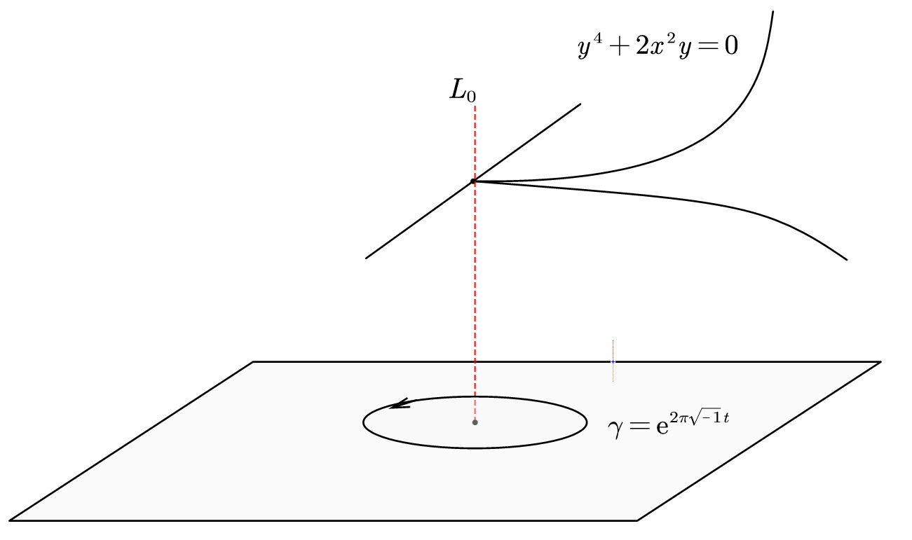
Hence the singular set $S$ is just one point, and the fundamental group $\pi_{1}(\mathbb{C}\setminus S,x_{0})$ is just $\mathbb{Z}$ . For each $x\in\mathbb{C}\setminus S$ , since the curve has degree 4, the fundamental group of the fiber is just

\pi_{1}(\mathbb{C}\setminus\{\text{4 points}\})\cong\mathbf{F}_{4}

Their generators will be denoted by $g_{1},g_{2},g_{3}$ , and $g_{4}$ .

Choose $\gamma(t)=e^{2\pi\sqrt{-1}t}\in\pi_{1}(\mathbb{C}\setminus S,x_{0})$ , the generator (see figure 7), the change on the fiber will give the braid as $\sigma_{1}\sigma_{3}\sigma_{2}\sigma_{1}\in B_{4}$ , see figure 8

Now, We can compute by (1):

	$\displaystyle g_{1}$	$\displaystyle=\sigma_{1}\sigma_{3}\sigma_{2}\sigma_{1}(g_{1})=g_{4}$
	$\displaystyle g_{2}$	$\displaystyle=\sigma_{1}\sigma_{3}\sigma_{2}\sigma_{1}(g_{2})=g_{1}g_{2}g_{1}^{-1}\Rightarrow g_{1}g_{2}=g_{2}g_{1}$
	$\displaystyle g_{3}$	$\displaystyle=\sigma_{1}\sigma_{3}\sigma_{2}\sigma_{1}(g_{3})=g_{4}$
	$\displaystyle g_{4}$	$\displaystyle=\sigma_{1}\sigma_{3}\sigma_{2}\sigma_{1}(g_{4})=g_{3}g_{4}g_{3}^{-1}$

By theorem 2.2, we finally know that

\pi_{1}\left(\mathbb{C}^{2}\setminus\left\{y(1+2x^{2}y)=0\right\}\right)\cong\pi_{1}\left(\mathbb{C}^{2}\setminus\left\{y^{4}+2x^{2}y=0\right\}\right)=\mathbb{Z}\oplus\mathbb{Z}

The first part is proved.

The generators in the $\pi_{1}\left(\mathbb{C}^{2}\setminus\left\{y(1+2x^{2}y)=0\right\}\right)$ can be found in the following way: The curve $x=1$ intersects the curve $y(1+2x^{2}y)=0$ at $q_{1}=(1,-1/2)$ and $q_{2}=(1,0)$ , let $\gamma_{1},\gamma_{2}$ be the meridians in the complex plane $\{(1,y)|y\in\mathbb{C}\}$ based at $(1,-1/4)$ and go around $q_{1},q_{2}$ by a small circle respectively. These $\gamma_{1},\gamma_{2}$ will be the generators.

To compute the Hamiltonian monodromy group, we will use the following fact

Lemma 4.1 ([10]).

$(1)$ . The 1-forms $\omega_{1},\omega_{2}$ :

	$\displaystyle\omega_{1}$	$\displaystyle=\left(\frac{\sqrt{-1}}{w}-\frac{x}{w(z+\sqrt{-1}x)}\right)dw-\frac{\sqrt{-1}}{\xi}d\xi$		(10)
	$\displaystyle\omega_{2}$	$\displaystyle=\frac{w}{z+\sqrt{-1}x}dw$		(10)

are holomorphic 1-forms defined on an open set of $M_{\mathbf{c}}$ where $z+\sqrt{-1}x\neq 0$ , and they can be extended analytically to the whole $M_{\mathbf{c}}$ .

$(2)$ . The following set

\Lambda_{\mathbf{c}}:=\left\{\left.\left(\int_{\Gamma}\omega_{1},\int_{\Gamma}\omega_{2}\right)\right|\Gamma\in H_{1}(M_{\mathbf{c}};\mathbb{Z})\right\}

is the period lattice of $M_{\mathbf{c}}$ . The generating vectors are $(2\pi,0)$ and $(u,v)$ , where

u=\int_{\gamma}\left(\frac{\sqrt{-1}}{w}-\frac{x}{w(z+\sqrt{-1}x)}\right)dw,\,v=\int_{\gamma}\frac{w}{z+\sqrt{-1}x}dw

here $\gamma$ is the generator of $H_{1}(\mathcal{R};\mathbb{Z})\cong\mathbb{Z}$ ( $\mathcal{R}$ is defined in (9)).

$(3)$ . The Hamiltonian monodromy matrices of the lattice $\Lambda_{\mathbf{c}}$ along $\gamma_{1},\gamma_{2}\in\pi_{1}(\mathbb{C}^{2}\setminus\mathcal{C})$ are the conjugations

\mathrm{Mon}(\gamma_{i})=P_{i}\begin{pmatrix}-1&0\\ -2&1\end{pmatrix}P_{i}^{-1},\,\,\,i=1,2

Then the monodromy group follows directly from lemma 4.1, and we refer to [10, §5] for a detailed proof. $\clubsuit$

Acknowledgement

The author would like to thank to Mr. Yunpeng Meng and Mr. Hongjie Zhou for the meaningful discussions, thank to Prof. Shanzhong Sun for his generous guidance, and thank to Prof. José I. Cogolludo-Augustín for his kind and patient explanation in using Zariski-van Kampen method.

Reference

[1] Johannes J Duistermaat. On global action-angle coordinates. Communications on pure and applied mathematics, 33(6):687–706, 1980.
[2] Otto Forster. Lectures on Riemann surfaces, volume 81. Springer Science & Business Media, 2012.
[3] Richard H Cushman and Larry M Bates. Global aspects of classical integrable systems, volume 94. Springer, 1997.
[4] Alain Albouy. Lectures on the two-body problem, 2002.
[5] Bruno Cordani. The Kepler Problem: Group Theotretical Aspects, Regularization and Quantization, with Application to the Study of Perturbations, volume 29. Springer Science & Business Media, 2003.
[6] MS Child. Quantum monodromy and molecular spectroscopy. Contemporary Physics, 55(3):212–221, 2014.
[7] RH Cushman, HR Dullin, A Giacobbe, DD Holm, M Joyeux, P Lynch, DA Sadovskií, and BI Zhilinskií. $\mathrm{CO}_{2}$ molecule as a quantum realization of the 1:1:2 resonant swing-spring with monodromy. Physical review letters, 93(2):024302, 2004.
[8] Alain Albouy and Vadim Kaloshin. Finiteness of central configurations of five bodies in the plane. Annals of mathematics, pages 535–588, 2012.
[9] Frits Beukers and Richard Cushman. The complex geometry of the spherical pendulum. Contemporary mathematics, 292:47–70, 2002.
[10] Shanzhong Sun and Peng You. Monodromy of complexified planar kepler problem. arXiv preprint arXiv:2209.00146, 2022.
[11] Daniel C Cohen and Alexander I Suciu. The braid monodromy of plane algebraic curves and hyperplane arrangements. Commentarii Mathematici Helvetici, 72:285–315, 1997.
[12] Enrique Artal Bartolo, Jorge Carmona Ruber, and José Ignacio Cogolludo-Agustín. Braid monodromy and topology of plane curves. Duke Mathematical Journal, 118(2):261–278, 2003.
[13] Phillip Griffiths and Joseph Harris. Principles of algebraic geometry. John Wiley & Sons, 2014.
[14] David Mumford. Tata Lectures on Theta II: Jacobian theta functions and differential equations. Springer, 2007.
[15] P Vanhaecke. Integrable Systems in the Realm of Algebraic Geometry. Springer, 2001.
[16] Arnaud Beauville. Holomorphic symplectic geometry: a problem list. In Complex and Differential Geometry: Conference held at Leibniz Universität Hannover, September 14–18, 2009, pages 49–63. Springer, 2011.
[17] Misha Verbitsky. Hyperkaehler and holomorphic symplectic geometry. arXiv preprint alg-geom/9307009, 1993.
[18] Nigel J Hitchin. The self-duality equations on a riemann surface. Proceedings of the London Mathematical Society, 3(1):59–126, 1987.
[19] José Ignacio Cogolludo-Agustín. Braid monodromy of algebraic curves. In Annales mathématiques Blaise Pascal, volume 18, pages 141–209, 2011.
[20] V Hansen. Braids and Coverings: Selected Topics. Cambridge University Press, 1989.
[21] Joan S Birman. Mapping class groups and their relationship to braid groups. Communications on Pure and Applied Mathematics, 22(2):213–238, 1969.
[22] Michele Audin. Hamiltonian monodromy via picard-lefschetz theory. Communications in mathematical physics, 229:459–489, 2002.
[23] Igor Reider. Toward abel-jacobi theory for higher dimensional varieties. In Algebraic Geometry: Proceedings of the International Conference held in L’Aquila, Italy, May 30–June 4, 1988, pages 287–300. Springer, 2006.

Zariski-van Kampen Method and Monodromy in Complexified Integrable Systems

Abstract

1 Introduction

Theorem 1.1 (Theorem 3.1 and Theorem 4.1).

2 Preliminaries

2.1 Complex Integrable System

Theorem 2.1 (Riemann Conditions, [13]).

Definition 2.1 (Complex integrable system, [14]).

Remark 2.1.

2.2 Braid Monodromy and Zariski-van Kampen Method

2.2.1 Braid Groups

Definition 2.2 ([20]).

Remark 2.2 (Pure Braids).

Example 2.1.

Example 2.2 (Artin representation).

Example 2.3.

2.2.2 Fundamental Group of the Complement of an Algebraic Curve

Remark 2.3.

Proposition 2.1 ([11]).

Theorem 2.2 (Zariski-van Kampen, [19]).

Example 2.4 (The Riemann surface of z\sqrt{z}).

Theorem 2.3 ([19]).

3 Complexified Spherical Pendulum

3.1 Complexification

3.2 Singular Set and Monodromy

Proposition 3.1 ([9]).

Theorem 3.1.

Lemma 3.1 ([9]).

Remark 3.1.

4 Complexified Planar Kepler Problem

4.1 Complexification

Proposition 4.1.

4.2 Singular Set and Monodromy

Proposition 4.2 ([10]).

Theorem 4.1.

Lemma 4.1 ([10]).

Acknowledgement

Reference

Example 2.4 (The Riemann surface of $\sqrt{z}$ ).