Zero, Normal and Super-radiant Modes for Scalar and Spinor Fields in Kerr-anti de Sitter Spacetime
Abstract
Zero and normal modes for scalar and spinor fields in Kerr-anti de Sitter spacetime are studied as bound state problem with Dirichlet and Neumann boundary conditions. Zero mode is defined as the momentum near the horizon to be zero: , and is shown not to exist as physical state for both scalar and spinor fields. Physical normal modes satisfy the spectrum condition as a result of non-existence of zero mode and the analyticity with respect to rotation parameter of Kerr-anti de Sitter black hole. Comments on the super-radiant modes and the thermodynamics of black hole are given in relation to the spectrum condition for normal modes. Preliminary numerical analysis on normal modes is presented.
-
August 2016
1 Introduction
The interactions of black holes with matter fields are fundamental and important in observational astrophysics. It is well-known that super-radiant phenomenon (outgoing intensity of matter fields becomes greater than ingoing intensity) can occur in rotating black hole spacetime. The successive occurrence of super-radiant phenomena leads to instability, which is called ”black hole bomb”. Especially Kerr-anti de Sitter (AdS) spacetime leads to successive super-radiant phenomena because it plays the role of the reflection mirror [1, 2, 3, 4].
Also the stability of BH is related to the BH thermodynamics [5, 6], which should be defined in equilibrium states. G. ’t Hoot introduced the brick wall model in order to study BH thermodynamics [7] by imposing Dirichlet boundary condition on the event horizon of BH. The boundary condition defines normal modes (i.e., bound states) of matter fields and the sum of normal modes determines the partition function and the entropy of BH. The Boltzmann factor of the matter fields in the brick wall model becomes ill-defined, if the super-radiance for rotating BH occurs [8].
The super-radiant phenomenon is also important relating to the recent works on the star motion [9, 10] and the radiation from axion [11, 12]. Here we list up important features of the super-radiant phenomena in rotating BH:
-
A.
The general condition of super-radiant phenomena for scalar fields is
(1.1) where , , and (defined in sec. 2.3) denote the frequency, momentum near the horizon, azimuthal angular momentum for scalar fields and angular velocity of BH, respectively [13, 14, 15]. Usually the super-radiant condition is under the implicit understanding that the frequency is positive . The super-radiance occurring under this condition is classified as type 1 [18].
- B.
-
C.
We studied the super-radiant phenomena of scalar and spinor fields as scattering problem in Kerr spacetime using the Bargmenn-Wigner formulation [18]. We derived the consistency condition for the current conservation relation among scalar and spinor fields, in accordance with the general super-radiant condition in equation (1.1).
-
C1.
The super-radiance with
(1.2) does not occur for neither scalar nor spinor fields, which is ”type 1” in our classification.
-
C2.
The super-radiance with
(1.3) does occur for both scalar and spinor fields, which is ”type 2”, in our classification.
-
C1.
Based on our previous works [18, 19], we study in this paper the bound state as normal modes for scalar and spinor fields in four dimensional Kerr-AdS spacetime and derive the physical spectrum condition for normal modes: . Key points are non-existence of zero modes and the analyticity of matter fields with respect to rotation parameter of BH.
The organization of this paper is as follows. In section 2, zero and normal modes are studied for scalar fields in Kerr-AdS spacetime. The spectrum condition for normal modes is derived. We shall show that the partition function in the brick wall model is well-defined and the super-radiant modes is type 2. In section 3, zero and normal modes are studied for spinor fields in Kerr-AdS spacetime. The spectrum condition for spinor fields is also derived, which turn out to be the same as that for scalar fields. In section 4, numerical analysis of normal modes for scalar fields in case of (mass of scalar fields) will be presented. Summary is given in section 5.
2 Scalar Fields in Kerr-AdS spacetime
In this section we study zero mode and normal modes as bound state problem for scalar fields in four-dimensional Kerr-AdS spacetime. Let us consider the Kerr-AdS metric in Boyer-Lindquist coordinates:
| (2.1) | |||||
where , , and denote the mass, rotation parameters of BH, and cosmological parameter, respectively. The event horizon is defined as the outer zero of factor .
The explicit expression of metrics are obtained from the line element in eq. (2.1) given in appendix A.
2.1 Scalar field equations
The Lagrangian and field equations for complex scalar fields in Kerr-AdS spacetime is given by:
| (2.2) | |||
| (2.3) |
where denotes the mass of scalar fields. If we write as
| (2.4) |
then the scalar field equations are separated into angular and radial field equations respectively:
| (2.5) | |||||
| (2.6) |
where , and denote the frequency, azimuthal angular momentum of scalar fields, and the separation parameter, respectively.
2.2 Normal modes and mode expansions
Now we study the normal modes as bound states with Dirichlet or Neumann boundary conditions on the horizon:
| (2.7) |
with asymptotic condition:
| (2.8) |
The following two identities can be obtained from eqs. (2.5) and (2.6):
| (2.9) |
for angular part and
| (2.10) |
for radial part.
Let us define as follows
| (2.11) |
Then from eqs. (2.9) and (2.10) we can obtain the following equations:
| (2.12) | |||||
| (2.13) |
which reduce to the real values of and the orthonormal relations:
| (2.14) |
Let us define the inner product notation of and as follows
The orthonormal relations are expressed:
| (2.15) |
with the eigenfunctions
where and denote set of quantum numbers.
Let us expand the scalar field and its conjugate momentum in eigenfunctions as follows
| (2.16) |
The inverse relations can be found to
| (2.17) |
using the completeness relations:
| (2.18) |
Note that any states, including quasi-normal modes and super-radiant modes, can express in terms of eigenfunctions due to the completeness relation (2.18).
Canonical quantization relations are given by
| (2.19) |
which lead to the quantization of creation and annihilation operators:
2.3 Conservation of energy and angular momentum
Energy and angular momentum of scalar fields are given by
| (2.20) |
which can be also written as
The effective energy of scalar field, as measured by the co-rotating observer, is given by
| (2.21) |
where
| (2.22) |
denotes the angular velocity of BH on the horizon .
Note that for normal modes near the horizon, we have ingoing and outgoing solutions with the momentum with respect to a radial variable as and . The effective frequency is the same in magnitude with the momentum because scalar field is treated as massless near the horizon:
| (2.23) |
2.4 Non-existence of zero mode and spectrum condition for normal modes
Now we consider the existence or non-existence of zero mode defined by . Radial equation for zero mode becomes:
| (2.24) |
where denotes the frequency of zero mode. The zero mode equation near horizon becomes from eq. (2.24):
| (2.25) |
where with . General solution of eq. (2.24) is given by, using the Frobenius method:
| (2.26) |
where denote integration constants. If we impose the Dirichlet boundary condition, then from eq. (2.26), we find that . Therefore non-trivial solution to eq. (2.25) which satisfies the Dirichlet boundary condition does not exist. We can also show the zero mode solution to eq. (2.25) does not satisfy the Neumann boundary condition either.
From this result we can derive the spectrum condition of normal modes for scalar fields with Dirichlet or Neumann boundary conditions as follows:
-
(i)
When the specific rotation parameter , the zero mode line is on and the allowed physical modes are in plane as in the standard scalar field theory in flat Minkowski spacetime.
-
(ii)
When , the zero mode is defined by the line in plane and the allowed physical modes should satisfy the spectrum condition:
(2.27) The reason is that any normal modes cannot across the zero mode line where the radial functions cannot satisfying the Dirichlet or Neumann boundary conditions. In this argument we take account of the analyticity with respect to rotation parameter under conditions that the outer horizon should be well separated zero of from other zeros and the rotation parameter should be less than the cosmological parameter for regularity of and .
Let us comment on super-radiant modes and the brick wall model.
-
(1)
We can apply the spectrum condition for normal modes to super-radiant modes because any modes can express in terms of eigenfunctions due to the completeness relation in eq. (2.18). Then allowed types of super-radiant modes taking account of general super-radiant condition given in equation (1.1) are the following two:
-
type 1
is unphysical and does not occur because this type contradicts with the spectrum condition of (2.27).
-
type 2
are physical which coincides with both equations (1.1) and (2.27).
In type 2 super-radiance, annihilation operators of particles with are understood as creation operators of antiparticles with as the interpretation in quantized field theory. Also, we mention that the results obtained here are consistent with our previous work basen on the Bargmann-Wigner formulation for scattering problem in Kerr spacetime [18].
-
type 1
-
(2)
The partition function in the Kerr-AdS black hole background spacetime becomes well-defined:
(2.28) considering the expression of effective energy (2.21) and the spectrum condition (2.27).
3 Spinor fields in Kerr-AdS spacetime
Next we consider zero and normal modes as bound states of massive spinor fields in Kerr-AdS spacetime. We study the spectrum condition and investigate the allowed type of super-radiant modes for spinor case, which can be compared with that for scaler case studied in the previous section.
In order to study the Dirac equation in curved spacetime, the local tetrads are introduced at each point of the general curved spacetime. The line element expressed in equation (2.1) is given as
| (3.1) |
The relation between the local tetrad and the general curved coordinate defines Viervein as , where the Greek letters () denote curved spacetime indices, and the Latin letters (i,j , …) denote local tetrads. The explicit expressions of Vierbeins for Kerr-AdS spacetime are given in appendix B.
3.1 The Dirac equation in Kerr spacetime
The Dirac equation in general curved spacetime is given by
| (3.2) |
where , , and denote the spin connection, the anti-symmetric product of Dirac gamma matrices, and the mass of spinor fields, respectively. The spin connections are divided into two terms:
| (3.3) |
whose derivation is in Appendix C. The first term of the right-hand side of eq. (3.3) is geometric in origin and the second term has spinorial origin. The totally anti-symmetric product of Dirac matrices is denoted by . Each term is calculated as
| (3.4) | |||||
| (3.5) |
Then the explicit form of Dirac equation in Kerr-AdS spacetime in the Boyer-Lindquist coordinate becomes:
| (3.6) | |||||
The representation of Dirac matrices are:
| (3.11) | |||||
| (3.16) | |||||
| (3.19) |
where are Pauli matrices.
With the ansatz
| (3.20) |
where denote the frequency and azimuthal quantum number, respectively, the Dirac equation becomes
| (3.21) | |||||
where the first term on the right-hand side of eq. (3.3) is eliminated. Furthermore, let us expand the spinor wave function in chiral eigenfunctions as follows:
| (3.22) |
with . Then the Dirac equation becomes
| (3.23) | |||||
where the second term on the right-hand side of eq. (3.3) is eliminated. Let be such that
| (3.28) | |||||
| (3.33) |
Then the Dirac equation reduces to the following set of the ordinary differential equations:
| (3.34) | |||
| (3.35) | |||
| (3.36) | |||
| (3.37) |
where is the separation parameter. The Dirac equations of the form (3.13)-(3.16) are consistent with other previous works for Schwarzschild and Kerr spacetime [20, 21, 22, 23, 24].
3.2 Non-existence of zero modes for spinor fields
Now we study zero mode for spinor field. Radial equations for zero mode become
| (3.38) |
where . Near the horizon, zero mode equations (3.17) become
| (3.39) |
where with . General solutions to eq. (3.18) are given by
| (3.40) |
where and are integration constants.
The Dirichlet and Neumann boundary conditions for spinor fields require the spacial component (in the present case, the radial component) of conserved current on the horizon to vanish:
| (3.41) |
where . The explicit expression for is given by
| (3.42) |
where we used eqs. (3.8), (3.10) and (3.12). There are two solutions of ,
| (3.43) |
which correspond to the Dirichlet and Neumann boundary conditions, respectively. 222 The Dirichlet and Neumann boundary conditions for spinor fields in eq. (3.22) are certified by the Bargmann-Wigner formulation too. Here a constant phase factor is introduced, where is in eq. (3.18). (Note that the additional phase factor reduces to unity in the massless limit: as ). The zero mode solution in equation (3.19) satisfies neither (i) nor (ii) in eq. (3.22). This means that the zero mode of spinor fields does not exist as physical states.
From the non-existence of zero mode for spinor fields we can derive the spectrum condition of normal modes for spinor fields satisfying as in the scalar field case.
As a consequence of the spectrum condition, type 1 super-radiance () cannot occur whereas type 2 super-radiance () does occur for spinor fields as well as scalar fields.
4 Numerical analysis on normal modes for scalar fields
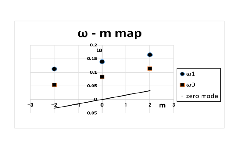
Now we present numerical analysis of normal modes for scalar fields in Kerr spacetime with the Dirichlet boundary condition and with special choice of parameter . In this case the separation parameter is set to the value . Parameters in the theory are chosen for the cosmological parameter and the black hole mass as and , and for the frequency, azimuthal quantum number of spinor fields as , . In Figure 1, the zero mode line, the ground state mode with respect to radial component denoted as and the first excited state modes as are shown. We can recognize that the normal modes with Dirichlet boundary condition on the horizon lie above the zero mode line and the spectrum condition is realized.
5 Summary
Zero and normal modes are studied for scalar and spinor fields in Kerr-AdS spacetime in case of the Dirichlet and Neumann boundary conditions.
-
S1
For zero mode (), radial eigenfunctions that satisfy the Dirichlet or Neumann boundary condition does not exist for both scalar and spinor fields.
-
S2
The spectrum condition for physical normal modes are in the range of , because (i) normal modes are in the positive omega region in no rotating cases and (ii) wave functions must be analytic with respect to the rotation parameter . The spectrum condition holds for both scalar and spinor fields.
-
S3
We apply the spectrum condition for normal modes (i.e., bound state problem) to the super-radiant phenomena, we find that the type 2 super-radiances ( and ) are possible for both scalar and spinor fields. Note that the type 1 super-radiances does not occur.
-
S4
The preliminary numerical analysis with the special choice of parameters: and supports the previous theoretical analysis discussed in sections 2 and 3.
-
S5
The partition function in brick wall model is well-defined because of the spectrum condition .
Note that the result on the super-radiance is consistent with our previous works where the Bargmann-Wigner formulation was applied to scattering problem for both bosons and fermions in Kerr spacetime [18], and normal modes for scalar fields in BTZ spacetime was studied analitically and numerically [26]. Notice also that as to type 2 super-radiance, the annihilation operators of particles with negative frequency and negative azimuthal quantum number correspond to the creation operators of antiparticles with positive frequency and positive azimuthal quantum number as in standard quantum fields theory. This interpretation supports the idea proposed by Penrose [25]. Type 2 super-radiance is natural in the classical picture of super-radiant phenomena in rotating spacetime.
Appendix A Metric in Kerr-AdS spacetime
The metric are obtained from the line element of Kerr-AdS spacetime in equation (2.1) as :
| (A.1) |
The determinant of metric is given as
| (A.2) |
Appendix B Vierbein in Kerr-AdS spacetime
The Vierbein in Kerr-AdS spacetime are obtained through the relation with the coordinate relation in equation (3.1):
| (B.3) |
The inverse Vierbein are obtained by the relation as
| (B.4) |
Appendix C Spin connection formula
The definition of the spin connection is obtained from the vierbein hypothesis:
| (C.5) |
as
| (C.6) |
where denotes the Christoffel’s 3-index symbol. Using the identity , the spin connection term in the Dirac equation (3.2) is written as
| (C.7) |
The first term on the right-hand side in eq. (C.3) is written in a compact form as
| (C.8) |
and the second term is written as
| (C.9) |
The sum of eqs. (C.4) and (C.5) is the spin connection formula in eq. (3.3).
References
References
- [1] W. H. Press and S. A. Teukolsky, Nature 238, 211 (1972).
- [2] S. Chandrasekhar, The Mathematical Theory of Black Holes, Claredon Press (1983).
- [3] V. Cardoso, O. J. C. Dias, J. P. S. Lemos and S. Yoshida, Phys. Rev. D70, 044039 (2004); V. Cardoso and O. J. C. Dias, Phys. Rev. D70, 084011 (2004).
- [4] H. Kodama, Prog. Theor. Phys. Suppliment 172, 11 (2008).
- [5] S.W. Hawking, Phys. Rev. Lett. 26, 1334 (1971).
- [6] B. Carter and S. W. Hawking, Commun. Math. Phys. 31. 161 (1973).
- [7] G. ’t Hooft, Nucl. Phys. B256, 727 (1985).
- [8] S. Mukohyama, Phys. Rev. D61, 124021 (2000).
- [9] V. Cardoso, R. Brite and J. C. Rosa, Phys. Rev. D91, 124026 (2015).
- [10] J. G. Rosa, arXiv: 1501.07605v1 (2015).
- [11] H. Yoshino and H. Kodama, Prog. Theor. and Exp. Phys. 043, E02 (2014).
- [12] H. Yoshino and H. Kodama, arXiv: 1505.00714v1 (2015).
- [13] J. D. Bekenstein, Phys. Rev. D7, 949 (1973).
- [14] W. G. Unruh, Phys. Rev. Lett. 31, 1265 (1973); Phys. Rev. D10, 3194 (1974).
- [15] S. Mano and E. Takasugi, Prog. Theor. Phys. 97, 213 (1997).
- [16] S. M. Wagh and N. Dadhich, Phys. Rev. D32, 1863 (1985).
- [17] S. Maeda, Prog. Theor. Phys. 55, 1677 (1976).
- [18] M. Kenmoku and Y.M. Cho, Int. J. Mod. Phys. A30, 1550052 (2015).
- [19] M. Kenmoku, arXiv: 0809.2634v3 (2008).
- [20] S. Chandrasekhar, Proc. R. Soc. Lond. A349, 571 (1976); The Mathematical Theory of Black Holes, London, Oxford University Press (1983).
- [21] F. Belgiorno and S. L. Cacciatori, J. Math. Phys. 51, 033517 (2010).
- [22] P. J. Mao, L. Y. Jia and J. R. Ren, Mod. Phys. Lett. A26, 1509 (2011).
- [23] H. Cebeci and N. Ozdemir, arXiv: 1212.310v1 (2012).
- [24] S. R. Dolen and D. Dempset, arXiv:1504.03190v1 (2015).
- [25] R. Penrose, Rerista del Nuovo Ciment 1, 252 (1969).
- [26] M. Kuwata, M. Kenmoku and K. Shigemoto, Class. Quant. Grav. 25, 145016 (2008); Prog. Theor. Phys. 119, 939 (2008).