ZMP support areas for multi-contact mobility
under frictional constraints
Abstract
We propose a method for checking and enforcing multi-contact stability based on the Zero-tilting Moment Point (ZMP). The key to our development is the generalization of ZMP support areas to take into account (a) frictional constraints and (b) multiple non-coplanar contacts. We introduce and investigate two kinds of ZMP support areas. First, we characterize and provide a fast geometric construction for the support area generated by valid contact forces, with no other constraint on the robot motion. We call this set the full support area. Next, we consider the control of humanoid robots using the Linear Pendulum Mode (LPM). We observe that the constraints stemming from the LPM induce a shrinking of the support area, even for walking on horizontal floors . We propose an algorithm to compute the new area, which we call pendular support area. We show that, in the LPM, having the ZMP in the pendular support area is a necessary and sufficient condition for contact stability. Based on these developments, we implement a whole-body controller and generate feasible multi-contact motions where an HRP-4 humanoid locomotes in challenging multi-contact scenarios.
Index Terms:
Contact stability, Humanoid locomotion, Zero-tilting Moment Point (ZMP)I Introduction
The Zero-tilting Moment Point (ZMP) is the dynamic quantity thanks to which roboticists solved the problem of walking on horizontal floors. One of its key properties is that dynamic stability, i.e. the balance of gravity and inertial forces by valid contact forces, implies that the ZMP lies in the convex hull of ground contact points, the so-called support area [1, 2]. The support area thus provides a necessary (non-sufficient) condition for contact stability on horizontal floors.
For locomotion, the second key property of the ZMP lies in its coupling with the position of the center of mass (COM). By keeping a constant angular momentum and constraining the COM to lie on a plane, this relation simplifies into the Linear Inverted Pendulum Mode (LIPM) [3, 4]. In the LIPM, the COM moves away from the ZMP under the linear dynamics of a point-mass at the tip of an inverted pendulum. The stabilization problem is then to control the position of the tip (COM) of the pendulum by moving its fulcrum (ZMP).
These two main merits, a geometric stability condition and linearized dynamics, are as well-known as the two main limitations of the classical ZMP: it does not account for friction, and it can only be applied when all contacts are coplanar. The latter results from the definition of the ZMP as the point on the floor. In a general multi-contact scenario, each contact defines its own surface and there is no single “floor” plane. In a classic survey paper [5], Sardain and Bessonnet stated the problem to address as follows:
The generalization of the ZMP concept [to the case of multiple non-coplanar contacts] would be actually complete if we could define what is the pseudo-support-polygon, a certain projection of the three-dimensional (3-D) convex hull (built from the two real support areas) onto the virtual surface, inside which the pseudo-ZMP stays.
In this paper, we construct the areas conjectured by Sardain and Bessonnet. Our first contribution is to characterize the ZMP support area generated by valid contact forces, with no other constraint on the robot motion. We call this set the full support area. Our analysis provides a geometric construction that allows for fast calculations. Also, contrary to the assumption that “friction limits are not violated” usually made in the literature, this area fully takes friction into account.
From a control point of view, locomoting systems usually regulate their linear and angular momenta, as examplified by the Linear Pendulum Mode where the robot maintains a constant COM height and moves with a constant angular momentum. These tasks limit the whole-body momentum of the system, which consequently shrinks the ZMP support area. The second contribution of this paper is an algorithm to compute the ZMP support area for the linear-pendulum mode, which we call pendular support area. The latter takes into account both friction and angular-momentum constraints on the robot motion.
Combining these two advances, we design a whole-body controller for humanoids locomoting on arbitrary terrains. Choosing a virtual plane above the COM, we regulate the robot dynamics around that of a linear non-inverted pendulum. We showcase the applicability of the controller by locomoting a model of the HRP-4 humanoid robot in a challenging multi-contact scenario involving a large step supported by a hand-on-wall contact.
The paper is organized as follows. In Section II, we review previous work and introduce background notions necessary to understand the present work. In Section III, we characterize the full support area. We then provide in Section IV an algorithm to calculate the pendular support area, which we apply to multi-contact locomotion in Section V. Concluding remarks are finally provided in Section VI.
II Background
II-A Previous work
II-A1 Stability criteria
on horizontal floors, the ZMP of dynamically stable motions lies within the convex hull of contact points (CHCP). However, when the robot makes contact with different non-coplanar surfaces, the ZMP can no longer be defined as a point on the “ground” and the CHCP has no established connection with dynamic stability. Various attempts have been made in the literature to overcome this difficulty.
One line of research [5, 6, 7, 8] conjectured that the CHCP (a 3D volume in general) conveys the stability condition, and consequently sought to define a new point lying within this volume. Both [6] and [8] assumed that the moments at centers of pressure and ZMP are all zeros, which is not the case in general111 Sardain and Bessonnet [5] pointed out that the term “zero moment point” is misleading, as the moment at these points has actually a non-zero component along the surface normal. They suggested that “zero-tilting moment point” would be a more proper name. and thus results in a point that may not exist even in situations where stability is possible. Harada et al. [7] considered the CHCP as a ZMP support volume when the robot makes two feet contact with a horizontal floor and hand contacts with the environment. They detailed how to project the support volume on the floor to obtain a ZMP support area. While their construction applies to the general case with non-zero angular momentum, like all approaches based on convex hull of contact points, it assumes infinite friction coefficients. In this paper, we will see how to construct support areas that also take friction into account.
A parallel line of research kept the ZMP in a plane but relaxed the constraint that it coincides with the floor [9, 10, 11, 12]. Kagami et al. [9] had the insight that the ZMP could be taken relative to any plane normal, yet still assuming that this plane should pass through all contact points, which restricted their scope to a maximum of three contacts points. Sugihara et al. [10] introduced the notion of “Virtual Horizontal Plane” (VHP) in which contact points are projected on a virtual plane via the line connecting them to the COM, and the convex hull of these points is then taken as support area. Shibuya et al. [11] took the idea further by considering a virtual plane above the COM, while Sato et al. [12] applied this idea to stair climbing. However, like CHCP, VHP support areas suppose infinite friction coefficients. The approach proposed in the present paper also uses a virtual plane and the linear pendulum mode, but our support areas fully account for friction, which makes them a necessary and sufficient condition for contact stability.
Breaking away from the notion of ZMP, another line of work has focused on building criteria that keep equivalence with full contact stability [13, 14, 15, 16, 17]. The seminal work by Saida et al. [13] impulsed a shift of paradigm from the ZMP to the gravito-inertial wrench. It also proposed to orient the virtual plane orthogonally to the resultant force, which reinstates the support area as convex hull of (projected) contact points – an idea that may have been overlooked by the literature so far. Next, Hirukawa et al. [14] constructed the first full stability criterion for the gravito-inertial wrench, yet with a high number of variables including all contact forces. Later developments [15, 16, 17] reduced these redundant variables to the gravito-inertial wrench using the double-description method. Compared to traditional ZMP solutions, this approach has the benefit of providing a full stability criterion, but at the cost of the non-linear dynamics of the gravito-inertial wrench. Furthermore, the nice geometric construction of the ZMP area is replaced by a considerably less intuitive six-dimensional cone. The method that we introduce in this paper reconciles full stability, linearized dynamics and a geometric support area.
II-A2 Control
when it comes to control, the use of the ZMP is historically tied to the LIPM, which was introduced in [4, 10] and used in a wealth of subsequent works [6, 7, 11, 12, 18, 19, 20, 21]. Kajita et al. [18] brought in the technique of model predictive control as a way to generate COM trajectories from desired ZMP positions. Harada et al. [19] proposed an analytical alternative with polynomial solutions for the coupled COM-ZMP trajectories. Recently, Tedrake et al. [21] exhibited a closed-form solution for the linear-quadratic regulator tracking a reference ZMP. However, all of these methods only apply to locomotion on horizontal floors.
Aiming for locomotion on rough terrains, Zhao et al. [22] extended the LIPM to a “Prismatic Inverted Pendulum” where the COM altitude is allowed to vary linearly, while Morisawa et al. [23] provided a wider derivation where the COM belongs to a general two-dimensional manifold. Rather than the ZMP, recent papers [20, 24] chose to control the Capture Point to stabilize the unstable dynamics of the LIPM. In terms of support areas, though, the question is the same for the Capture Point and the ZMP and was not addressed by these developments. With the method proposed in the present paper, we realize a control system with marginally stable dynamics using the ZMP as control point and a linear pendulum mode. The benefit of our approach compared to these previous works is that we are able to derive at the same time the support area corresponding to our control variable.
As with stability criteria, solutions breaking away from control points were also explored in the whole-body control literature. The main alternative is to regulate contact forces directly, resulting in force distribution schemes where desired contact forces and torques are tracked by a whole-body controller [14, 25, 26, 27, 28]. Force objectives can express whole-body tasks, such as tracking of desired COM or angular momentum, as well as local ones, such as minimizing friction forces [27] or end-effector torques [26]. Notably, Righetti et al. [28] characterized the class of force-distribution controllers for linear-quadratic objectives in the absence of inequality constraints. Overall, force distribution schemes yield fast computations and can cope with arbitrary contact conditions, but they lack the foresight and intuition of methods based on control points and support areas. Indeed, for locomotion, support areas provide both reachable COM locations and a stability margin (the point-to-boundary distance). Finding such indicators in the high-dimensional contact-force space is still elusive. In recent developments, [29, 30] added a level of foresight to their contact-force controllers via model-predictive control, while Zheng et al. [31] constructed a metric that can be used as wrench-space stability margin. In the present paper, we show that support areas can be derived in arbitrary multi-contact configurations as well, providing both COM reachability and stability margins suitable for locomotion.
II-B Newton-Euler equations
Let and represent the total mass and center-of-mass (COM) of the robot, respectively. We write the vector of absolute coordinates of a point and denote by the origin of the absolute frame (so that ). For a link , define:
-
•
the total mass of the link;
-
•
the vector of absolute coordinates of its COM ;
-
•
its orientation matrix in the absolute frame;
-
•
its angular velocity in the link frame;
-
•
its inertia matrix in the link frame.
The linear momentum and angular momentum of the robot, taken at the COM , are defined by:
| (1) | |||||
| (2) |
The fundamental principle of dynamics states that the rate of change of the momentum is equal to the total wrench of forces acting on the system, that is:
| (3) |
where denotes the gravity force, the contact point and the contact force exerted by the environment on the robot at . Equation (3) is called the Newton-Euler equations of the system, sometimes also referred to as “dynamic balance” or the “dynamic equilibrium”. It can be equivalently derived from Gauss’s principle of least constraint, and corresponds to the six unactuated components in the equations of motion of the system robot environment [32].
Define the gravito-inertial wrench, taken this time at :
| (4) |
Define similarly the contact wrench:
| (5) |
The Newton-Euler equation (3) can be written in terms of these two wrenches as:
| (6) |
This formulation separates spatial accelerations (), that are usually measured by inertial measurement units, from interaction forces with the environment (), usually measured by force sensors. Since the two wrenches are simply opposites, we will only use the contact wrench in the following calculations, dropping the superscript to alleviate notations.
II-C Contact stability
We assume that all contacts between the environment and the robot are surface contacts, i.e. contacts between a flat surface of the robot and a flat surface of the environment. Wrenches exerted on each contacting link are then fully described by applying contact forces at the vertices of the contact polygon [33], which warrants the formulation by contact points that we have followed so far. Define the contact normal at as the normal to the contact surface pointing from the environment towards the contacting link. Under Coulomb’s model of dry friction, contact forces lie inside a friction cone directed by :
| (7) |
Frictional constraints restrict the range of contact wrenches that the robot can generate without breaking any contact: when each contact force lies in a cone , the contact wrench lies in the Contact Wrench Cone (CWC) projected from all ’s via the mapping (5). Because of the connection (6), the gravito-inertial wrench belongs to Gravito-inertial Wrench Cone (GIWC) . This link between feasible motions and keeping contacts is embodied by the notion of contact stability:
Definition 1 (Weak contact stability [34, 35]).
A motion of the robot is (weak-contact) stable if and only if the contact wrench it generates belongs to the CWC.
Weak contact stability is the underlying stability criterion used in recent multi-contact developments [14, 15, 16, 17]. Static stability [36] corresponds to contact stability when the whole-body momentum is zero. Note that the term “stability” is used here in the sense defined by Pang and Trinkle [34]. It should not be confused with the (a-priori unrelated) notion of Lyapunov stability.
II-D Linearized wrench cones
We linearize the quadratic constraint (7) by approximating friction cones by friction pyramids . Denoting by the ray vectors of the latter, the constraint becomes:
| (8) |
The set of ray vectors is known as the span representation of the pyramidal cone. It can be computed directly from the contact frame and friction coefficient . For example, the expression of a four-sided pyramid is , with an orthonormal contact frame, where the normalization by is added to make the friction pyramid an inner approximation of the friction cone. Injecting (8) into Equation (5) yields a span representation for the contact wrench cone:
| (9) |
Let us define . After re-indexing the couples into a single index (counting the same contact point multiple times accordingly), we get:
| (10) |
We have thus obtained the span representation of the CWC. A motion is weak-contact stable if and only if its contact wrench can be written as (10) for a certain set of coefficients .
III Full ZMP support area
Let be a fixed unit space vector, not necessarily aligned with the gravity vector. The Zero-tilting Moment Point (ZMP) is a point where the moment of the contact wrench aligns with [5], that is, . Consequently,
| (11) | |||||
| (12) |
We are interested in computing the ZMP in the plane that contains and that is orthogonal to , hereafter denoted by . The relation is expressed by , so that the equation above becomes:
| (13) |
On horizontal floors, is taken on the floor and is upward vertical, so that coincides with the floor plane. However, in what follows we assume that can be located at an arbitrary fixed position in space, while can be an arbitrary unit vector.
III-A Construction of the full support area
Equation (13) presents the ZMP as a two-dimensional projection of the contact wrench . Since contact stability is characterized by the CWC, we define the support area of the ZMP as the image of the CWC by this projection:
Definition 2 (Full support area).
The full support area of the ZMP in the plane is the image of the CWC by the projection (13):
| (14) |
The key idea to calculate this area is to use the span representation (10) of the CWC, which enables rewriting Equation (13) as
| (15) |
Next, define the points by:
| (16) |
and denote by the virtual pressure of the contact force generator through the virtual plane. Then,
| (17) |
On horizontal floors, and all contact forces point upwards, so that all pressures are positive. This makes the ZMP a convex combination of the ’s from Equation (17). Furthermore, Equation (16) simplifies to , i.e. , the vertices of the support area coincide with contact points. Our definition of the full support area therefore coincides with the conventional support area on horizontal floors.
In general, however, virtual pressures can be either positive or negative.222We assume is chosen so that none of them is zero, which is easy to do since there is only a finite set of generators . Let us then partition the set of generator indices into and . For any , denote by and define
| (18) | |||||
| (19) |
Equation (15) becomes
| (20) |
Define the positive-pressure polygon as the convex hull of ’s for : , and define the negative-pressure polygon similarly. Equation (20) can be rewritten as
| (21) |
where , , and . Next, let
| (22) |
denote the Minkowski difference of and . It is a polygon as difference of two polygons, so that it admits a span representation as convex hull (conv) of a set of vertices. We can now characterize the support area as follows:
Proposition 1.
If all virtual pressures have the same sign, then the full support area is the convex hull of the vertices . Otherwise, when both and are nonempty, let
| (23) |
denote their Minkowski difference. The full support area is then the reunion of two polygonal cones and given by
| (24) | |||||
| (25) |
In particular, when and intersect with nonempty interior, the full support area spans the whole virtual plane .
Proof:
(Note that this proof is quite formal and may be skipped by first-time readers.) The main idea of the proof is to combine pairs of points in to generate rays in and . Let us first clear out simple cases. When all ’s are positive (), Equation (17) shows that is a convex combination of the vertices of , where the weights can be chosen freely, so that . The case where is treated identically. Next, suppose that both and are nonempty. Equation (21) can be reformulated as
| (26) |
where (resp. ) is the weight of (resp. ) in Equation (21). Therefore, the set of points defined by this equation is
| (27) |
Given the orderings of and , we can further simplify the ratios into a single positive scalar, so that with
| (28) | |||||
| (29) |
The set is a convex polygon as Minkowski difference of two convex polygons. To conclude, we show that . The inclusion is straightforward from (28). Now, let
| (30) |
denote any point in . Define
| (31) |
One can check that , where belongs to as convex combination of two points from this convex polygon. Thus , which establishes the converse inclusion .
Finally, note how, when has non-empty interior, contains a neighborhood of the origin. For any pair of points , this implies that there exists a scaling such that . Then, as , we have . Since was taken arbitrarily in the virtual plane, this establishes that , i.e. the support area spans the whole virtual plane. ∎
The geometric construction given by Proposition 1 provides fast computations of the full support area. In particular, it is faster to use this approach than to project the CWC computed by polyhedral duality methods [17]. (A comparison of computation times for both approaches is reported in Table I.)
III-B Geometric properties
Proposition 1 gives the span representation of the full support area. By construction, this area depends only on contact locations and on the choice of the virtual plane . The latter involves the choice of a fixed point , but we will now see that the location of this point only matters as far as it defines the virtual plane of the ZMP.
Proposition 2.
The support area does not depend on the coordinates of the reference point in the virtual plane .
Proof:
By definition of the support area,
| (32) |
where ranges over the CWC. Now, choose a point and consider
| (33) |
Given a contact wrench , we have
| (34) | |||||
| (35) |
Thus, , and since the wrench we considered is arbitrary, we have shown that . ∎
By contrast, the support area does change for displacements of along the plane normal . Let us analyze the impact of this remaining coordinate by relaxing the assumption that . We now denote by the coordinate of the virtual plane, so that and . On a horizontal floor, and correspond to the altitude of the ZMP and COM, respectively. Given Proposition 2, we can write the virtual plane . The definition of the ZMP yields:
| (36) |
And repeating the step from Equation (16),
| (37) | |||||
| (38) |
We see from this equation that the vertices are located at the intersection between the plane and the ray of the linearized friction cone, which establishes that:
Proposition 3.
The vertices of the support area are located at the intersection between the virtual plane and the rays of the friction cones.
Proposition 4 (Polygonal case).
When all virtual pressures have the same sign, the support area is the convex hull of the intersections between linearized friction cones and the virtual plane.
This result is coherent with the horizontal-floor setting where the virtual plane intersects friction cones at their apexes (i.e. at contact points) and virtual pressures are all positive from contact unilaterality. A condition similar to the positivity of virtual pressures was also observed by Saida et al. (Proposition 4.1 in [13]) for some plane components of the contact wrench.
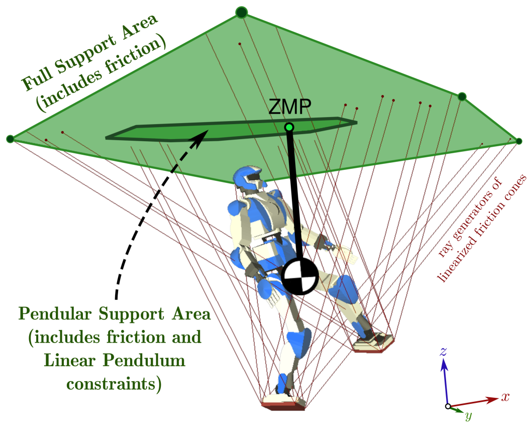
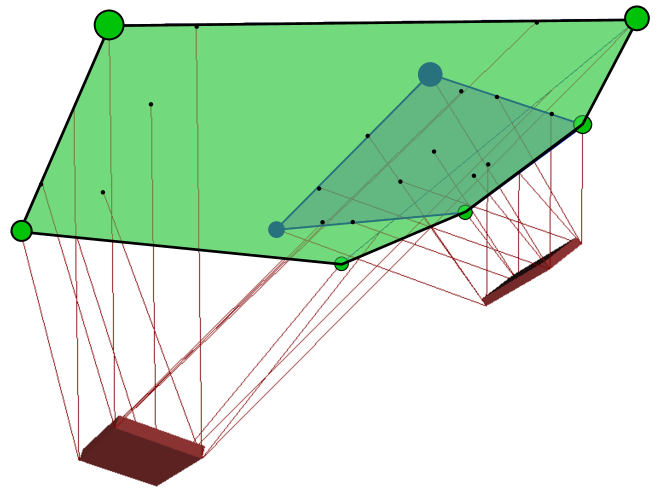
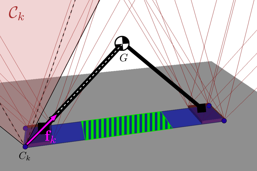
Figure 2 illustrates the geometric construction in the polygonal case. The support area (in green) is the convex hull of black points projected from friction rays (red lines). Alternatively, each individual contact surface projects its own support polygon (blue polygon in Figure 2), and the ZMP support area is the convex hull of these individual polygons. This second construction can be useful for contact planning, where the quality of contact candidates can be assessed by the expansion that they bring to the support area.
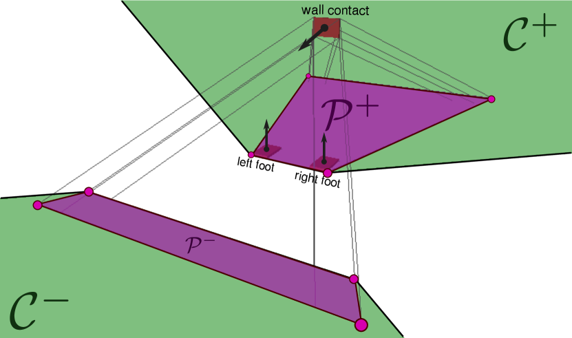
Figure 3 shows a configuration where the support area is the union of two polygonal cones. In this setting, the robot has its two feet on a horizontal floor, and pushes its hand on a wall in front of it. The positive cone illustrates how the wall contact expands the conventional support area between the two feet, while the negative cone reveals that a second support area appears behind the two floor contacts. This new area results from the ability for the robot to generate downward forces at the wall contact.
Finally, let us determine in which cases a polygonal ZMP support area can be found, which boils down to finding a suitable vector .
Proposition 5.
Either contact forces can generate any arbitrary resultant force or one can find a plane normal such that the support area is polygonal.
Proof:
Let denote the cone positively spanned by the ’s. Then, the condition is equivalent to , where is the dual cone of defined by
| (39) |
The set of solutions can be computed from . In particular, if and only if , i.e. the ’s positively span the whole space. ∎
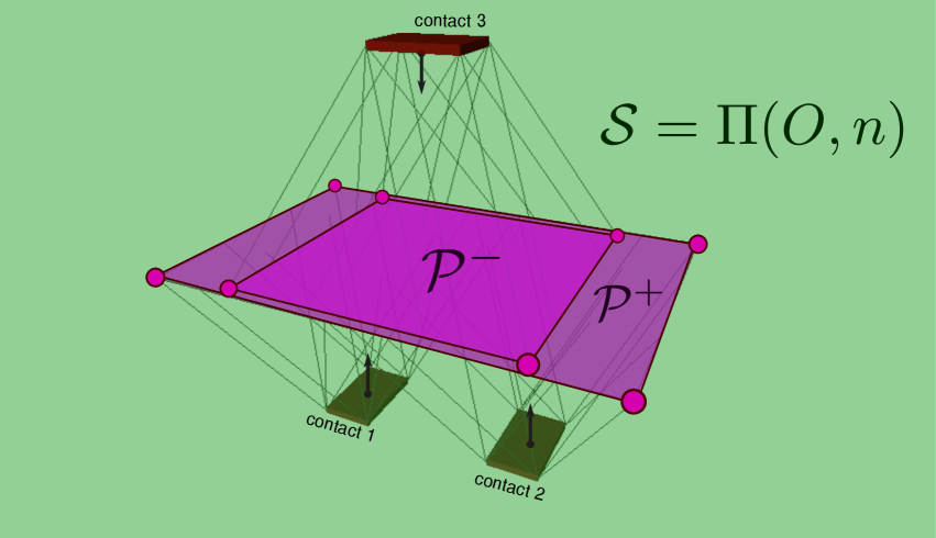
Figure 4 provides an example where contacts are in force closure. As they can generate arbitrary contact wrenches, the support area spans the whole virtual plane. Note that being able to generate arbitrary forces is a weaker condition than force closure, which usually assumes that contact forces can generate arbitrary resultant forces and momenta.
Excluding such configurations, from Proposition 5 one can choose such that for all resultant forces generated by valid contacts. This is desirable insofar as it eliminates potential singularities where the ZMP would be undefined (13). In the classical horizontal-floor setting, taking as the floor normal is an example of such a solution.
III-C Relation with the whole-body momentum
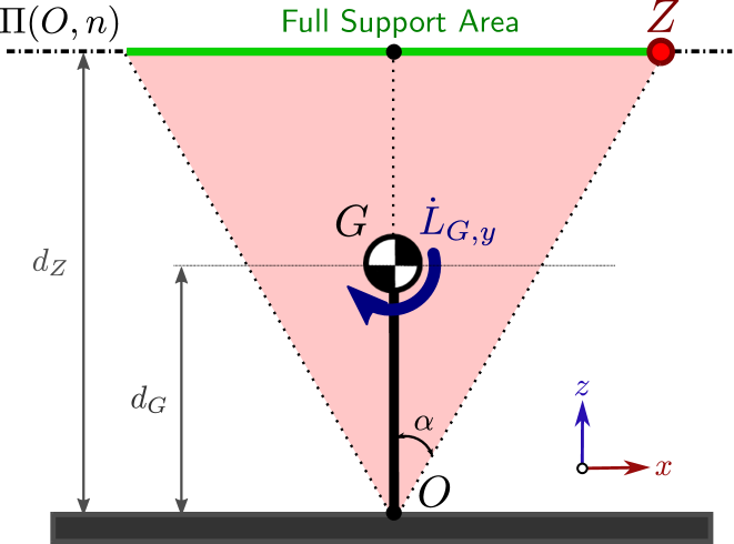
The full support area describes the ZMPs sustainable by valid contact forces. As such, it does not take into account kinematic and dynamic limitations of the robot itself, in particular the limited changes in whole-body momentum that the robot can generate around its COM by moving its limbs. Consider the simple example depicted in Figure 5, with a single point contact. According to Proposition 4, the full support area is given by the intersection of the friction cone with the virtual plane . To generate a ZMP , the robot needs to change its angular momentum around the COM by
| (40) |
Thus, ZMPs close to the boundary of the full support area () tend to generate higher angular momenta, a phenomenon which is amplified by the altitude of the virtual plane. In practice, legged robots cannot generate a arbitrary angular momenta, as torque limits and their bounded range of motion yield additional constraints, which in turn restrict the ZMPs that the robot can generate. One way to take these limitations into account is to put additional constraints on the whole-body momentum, as we will now see with the linear pendulum mode.
IV Pendular ZMP support area
From a control point of view, the strong point of the ZMP lies in its direct relationship with the acceleration of the COM. This can be seen with a suitable rewriting of the Newton-Euler equations of the system:
Proposition 6.
The COM acceleration, ZMP position and angular momentum are bound by the equation:
| (41) |
where is the gravity vector.
Proof:
IV-A Linear pendulum mode
The Linear Pendulum Mode (LPM) is a particular mode of Equation (41), obtained by regulating the COM altitude and the angular momentum to constant values:
Definition 3 (Linear Pendulum Mode (LPM)).
Provided with a normal vector , the linear-pendulum assumptions are:333 Strictly speaking, our definition includes both and , while only the former is necessary to realize the linear pendulum mode.
| (45) | |||||
| (46) |
When , the COM is above the virtual plane with respect to the plane normal. In such situations, Equation (41) yields the well-known linear inverted pendulum mode (LIPM) [4, 10]:
Proposition 7 (Linear Inverted Pendulum Mode (LIPM)).
Assume that , and define . The COM acceleration in the LPM is then related to the ZMP by:
| (47) |
The LIPM was a necessity in previous works as the ZMP was assumed to lie on the floor below the COM. But now that the virtual plane coordinate can be chosen freely, we may also consider the case where , i.e. taking the virtual plane above the COM. In this case, Equation (41) yields a linear non-inverted pendulum:
Proposition 8 (Linear Non-inverted Pendulum Mode (LNPM)).
Assume that , and define . The COM acceleration in the LPM is then related to the ZMP by:
| (48) |
The behavior of the ZMP with respect to COM acceleration differs between the two modes. In the LIPM, the ZMP is a repulsor of the COM: when it is maintained at a fixed position, the COM is “pushed away” from it and diverges to infinity. When selecting a virtual plane below the center of mass , ZMP trajectories will therefore follow the COM when it accelerates, and precede it when it decelerates.
In the LNPM, the ZMP is a marginal attractor of the COM: when it is maintained at a fixed position, the COM will “orbit” around it (yet without asymptotic convergence, as there is no damping term in Equation (48)). In a virtual plane above the center of mass (), ZMP trajectories will therefore precede the COM when it accelerates, and follow it otherwise.
These two complementary behaviors reflect the fact that, in the LPM, the resultant contact force always points from the COM to the ZMP. In what follows, we choose to take the virtual plane above the center of mass and use the LNPM.
IV-B Shrinking of the support area
Previous methods [9, 10, 18, 7, 11, 12] applied the LIPM using the convex hull of contact points (CHCP) as ZMP support area. By Proposition 4, when all contacts are coplanar the CHCP is the full support area. However, it turns out that the constraints (45)-(46) of the linear-pendulum mode shrink the ZMP support area.
This can be seen as follows. Suppose that the ZMP is located at a vertex of a given contact polygon. The resultant contact force must then be realized as one contact force applied at , while all other contact forces for . (From Equation (17), implies that only the ’s corresponding to can be strictly positive.) However, in the LPM the contact force is also directed from to . Hence, the ZMP support area cannot be the CHCP as soon as the COM lies outside of the friction cone of at least one ground contact point. An example of such situation is when a biped robot stretches its legs, as depicted in Figure 6.
Methods that take the Convex Hull of Contact Points (CHCP) as ZMP support areas rely by construction on the assumption of “infinite friction” to rule out such cases, at the cost of being problematic for locomotion on low-friction floors (apart from sliding, foot yaw rotations due to insufficient friction have also been observed and studied [37, 33]). This assumption explains why the shrinking of the ZMP support area in the LPM was not highlighted in previous works.
IV-C Computation of the pendular support area
In this section, we assume that , the upward vertical (opposite to gravity) unit vector. We now propose an algorithm to compute the pendular support area based on the double-description method [38]. It turns out that computations of this set are very similar to that of the COM static-equilibrium polygon. We explain both calculations here.
IV-C1 Static-equilibrium polygon
In static equilibrium, the equations on the contact wrench are:
| (49) | |||||
| (50) | |||||
| (51) |
By expanding the triple product in Equation (50), we can rewrite them equivalently as:
| (52) |
| (53) |
In concise form, these two equations can be written:
| (54) | |||||
| (55) |
Consider the stacked vector of contact forces . Linearized friction cones are given by linear inequalities . For instance, four-sided friction pyramids can be formulated as
| (56) |
Combining all ’s in a block diagonal matrix yields an inequality . Meanwhile, Equation (5) provides a linear mapping from contact forces to the contact wrench, where is the so-called grasp matrix. Then, the set of valid contact forces in static equilibrium is given by:
| (57) | |||||
| (58) |
This expression of a polytope by linear inequalities is known as the half-space representation. By the Minkowski-Weyl theorem [38], all polytopes can be equivalently written in terms of linear inequalities (half-space representation) or in terms of vertices and rays (span representation). The double description method [38] provides a “black-box” algorithm to convert between one representation and the other. Using this tool, one can compute the span representation of this set as:
| (59) |
where , and the ’s are computed vertices. The span representation of the stability polygon is finally given by
| (60) |
In the case of static stability, the solution is always a polygon, so there is no need to consider rays in this span representation. Note that this method for computing the COM static-equilibrium polygon by double-description is different from the recursive polytope projection algorithm [36].
IV-C2 Pendular support area
the Equations (45)-(46) of the LPM are written, in terms of the contact wrench:
| (61) | |||||
| (62) | |||||
| (63) |
where m.s-2 is the gravity constant. Taking the resultant moment rather than , one can rewrite the equations above as:
| (64) |
| (65) |
Equation (64) results from (61)-(62), while Equation (65) is a reformulation of (63).
Contrary to the previous setting, where the COM position resulted from the contact wrench in static equilibrium, we now assume that is known (e.g. measured from the instantaneous robot state). In concise form, the two equations above can be written:
| (66) | |||||
| (67) |
where the matrices and vectors now depend on . From there, the computations are the same as for static stability: the set of valid contact forces is given by
| (68) | |||||
| (69) |
Using the double description method, one can compute the span representation of this set as
| (70) |
where , and the ’s (rep. ’s) are the computed vertices (resp. rays). The span representation of the pendular support area is finally given by
| (71) |
Similarly to the full support area, the pendular area can be either conical or polygonal. Compared with the full support area or static-equilibrium polygon, it depends not only on the set of contacts , but also on the instantaneous position of the COM. Yet, where the full support area yields only a necessary condition for contact stability (it is a 2D projection of the 6D contact wrench, the remaining four components being unconstrained), the pendular support area gives a condition both necessary and sufficient under the LPM (the four other components of the contact wrench being determined by equality constraints).
V Experiments
V-A Trajectory generation
We now design a trajectory generator for ZMP-COM trajectories based on the model-preview control formalism introduced in previous works [18, 30]. We use the ZMP as a command and COM as the output variable. First, we define the support of the ZMP trajectory as a line segment:
| (72) |
where (resp. ) denotes the initial (resp. final) ZMP position. Assuming that its initial velocity is zero, the COM follows a parallel line segment :
| (73) |
where . Next, define the state of the control problem by and its command by the linear position of the ZMP. Discretizing the time interval into steps of duration , the system’s dynamics become
| (76) | |||||
| (79) |
Let and . Applying (76) repeatedly, we build the matrices and such that . We assume that the system starts with zero COM velocity, so that and .
We formulate the trajectory generation problem as a Quadratic Program (QP) as follows:
| Objective: | |||
| Constraints: | |||
The objective is the weighted sum of two terms:
| (80) | |||||
| (81) |
The first one minimizes COM accelerations while the second regularizes the ZMP trajectory. The weights of the cost function are set to and . Meanwhile, the constraints ensure respectively that:
-
•
the ZMP belongs to the line segment
-
•
the COM ends at the destination point with zero velocity ,
-
•
the ZMP also ends at the destination point .
The solution to this QP provides a ZMP trajectory , which is then integrated into a COM trajectory by applying (48). We also added a damping term at this stage to smooth out undesired COM oscillations. On a side note, set aside the two regularization objectives, this optimization problem falls under the framework of Time-Optimal Path Parameterization (TOPP) [39, 40]. One could then trade smoothness of COM accelerations for Admissible Velocity Propagation (AVP), allowing for the integration into a kinodynamic planner of COM trajectories [41].
With this method, contact stability is mostly enforced by checking that the segment lies inside the pendular support area computed for the extremities and of the segment. However, the COM moves as the robot performs the motion, which affects both the position and shape of the pendular support area. This phenomenon can have two undesired outcomes:
-
•
the area becomes empty: we observed empirically that this would only happen when the COM is far away (e.g. more than one meter) from contacts, and was not a threat in practice.
-
•
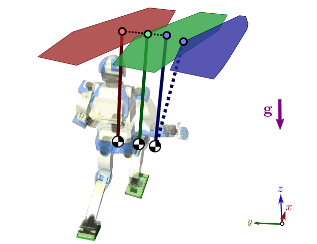
the area constraints the COM motion toward divergence: past a certain COM-to-contacts distance, the support area slants away from contacts, in a way such that it contains no ZMP that could bring the pendulum back above contacts.
Figure 8 illustrates this phenomenon. In practice, ensuring that the ZMP is well within the support area computed at the beginning and end of the segment was enough to rule out both undesirable outcomes.
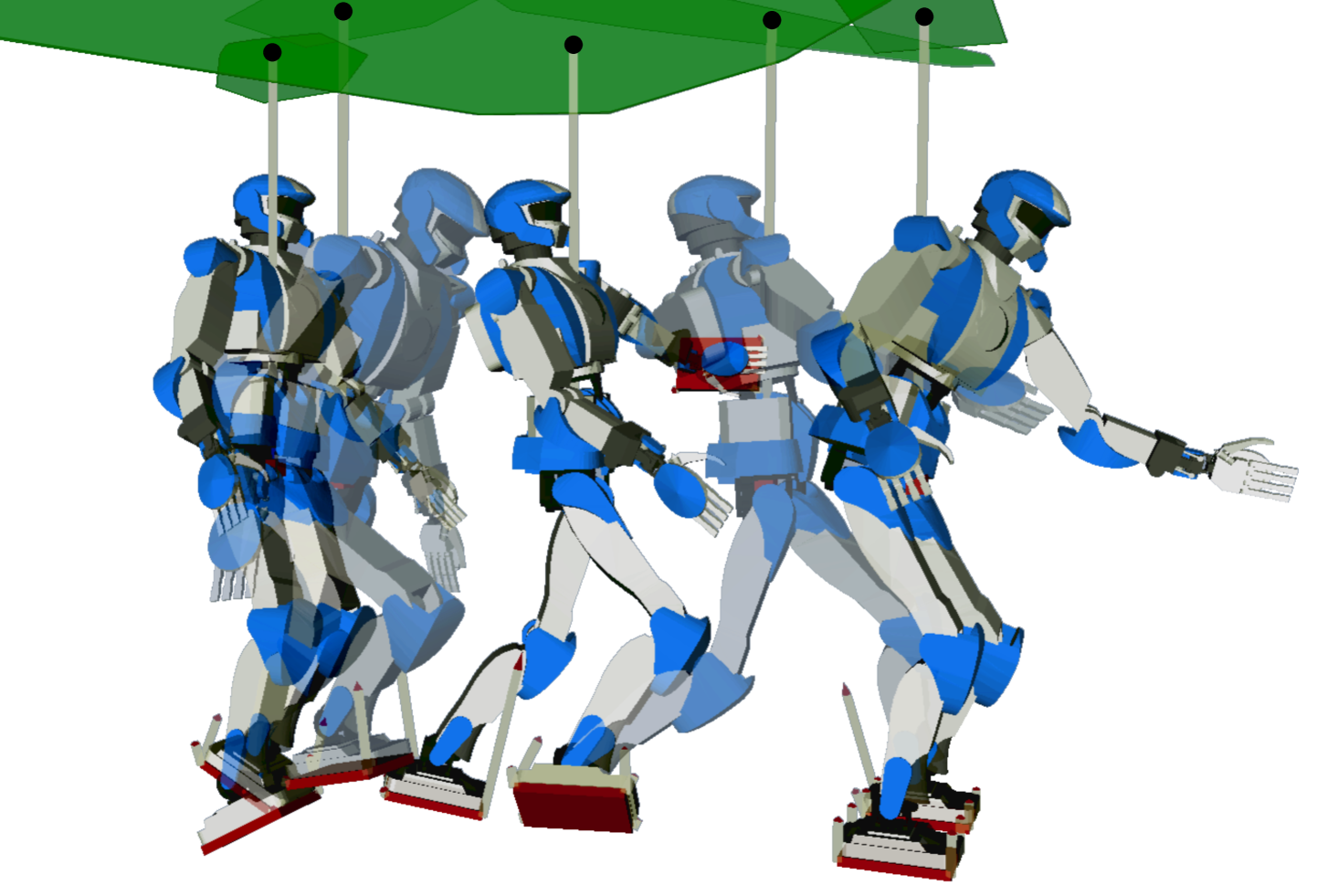
V-B Long stride while leaning on a wall
We implemented the whole pipeline described so far to generate multi-contact motions for a model of the HRP-4 humanoid robot. The scenario is depicted in Figure 9. The robot has to step on inclined platforms in order to reach its goal configuration on the right. Because there is no platform for its left foot in the middle of the course, the only way for it to complete the task is to put its left hand on the elevated “wall” platform while pushing with its right foot on the opposite tilted surface. Relying on these two simultaneous contacts, the humanoid can perform a long stride which would have been impossible to achieve in single-support.
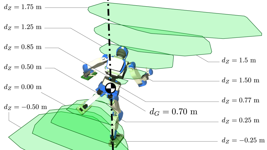
As input given to solve this scenario, we assume that a contact planner provides a sequence of stances, where a stance provides both a reference position of the COM and a set of contact points . The first stage of our solution computes stance-to-stance COM trajectories. To move from to stance , the controller considers the line segment . The trajectory generator is called if this segment is included in the pendular support area for the initial COM position. Otherwise, is increased until the segment is included in . This condition is easy to fulfill in practice, as we observed that the region grows like the section by the plane of a cone passing through (see Figure 7). In the motion depicted in Figure 9, this process lead us to take the virtual plane one meter above the center of mass of the humanoid (HRP-4 is 1.5-meter tall). Although contact planning was done by hand in this experiment, we also used the pendular support area to select COM positions from contact locations , by enforcing that the ZMP at the vertical of lies well inside .
Once a reference COM trajectory has been computed, we generate whole-body joint-angles by differential inverse kinematics (IK) under the following constraints, by decreasing task weight:
-
1.
tracking of contacting end-effector poses,
-
2.
tracking of COM trajectory,
-
3.
tracking of free end-effector poses,
-
4.
minimum variations in angular momentum
-
5.
preferred values for some joint-angles.
We applied our own IK solver for the task, which is released in the pymanoid library.444https://github.com/stephane-caron/pymanoid Similarly to [26], this solver relies on a single-layer QP problem, using the above cost function and a set of inequality constraints
| (82) |
to limit joint velocities. Gains and weights used in the simulations are reported in Table II, while other simulation parameters are given in Table III. Implementation details can be checked in the library and source code released with the paper (see the motion_editor distributed in [42]).
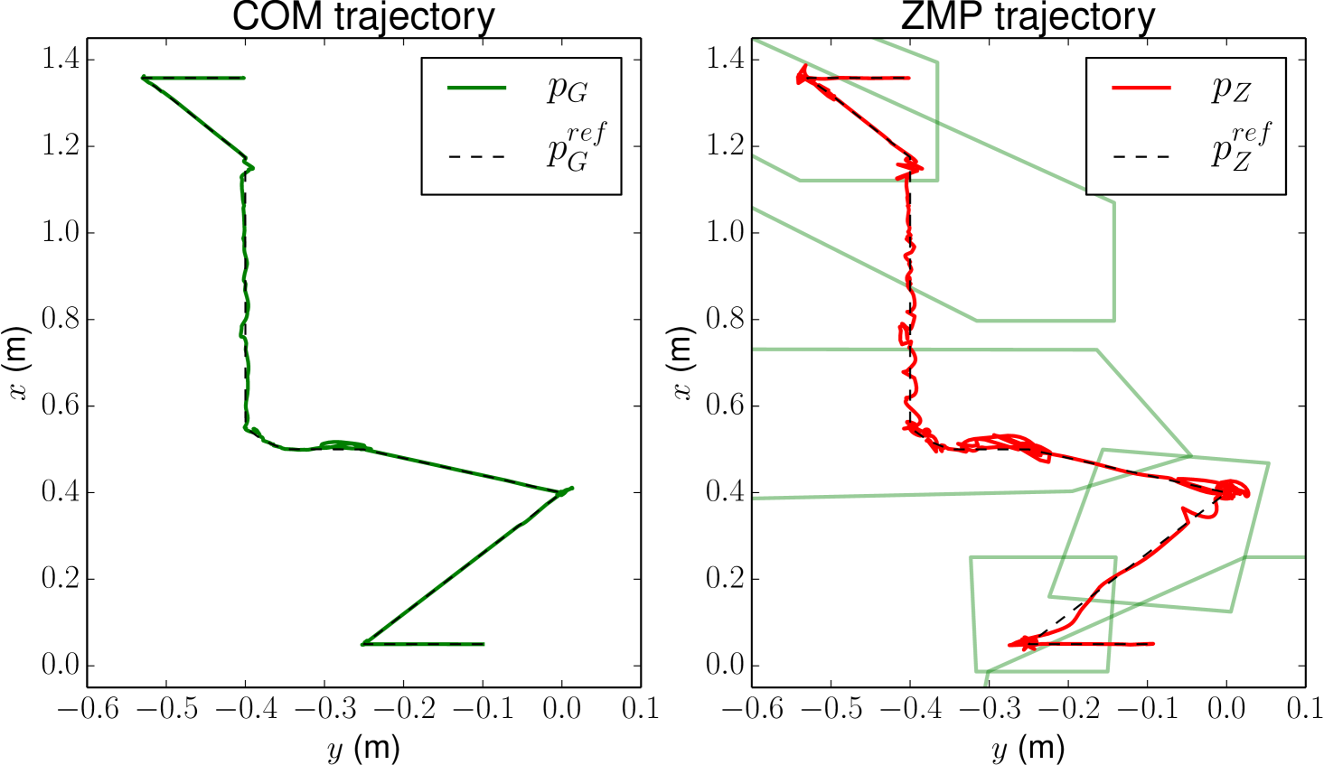
ZMP tracking is not an explicit task in the list above, and is realized as a side effect of the COM tracking task. The latter comes second in the hierarchy of the differential IK solver and is therefore not fulfilled perfectly, as illustrated in Figure 10. The same holds for the task , which has an even lower rank in the hierarchy. Yet, ZMP deviations in the generated trajectory are small enough and one can check that the ZMP always stays well within the pendular support area (see the accompanying video). We cross-validated the contact-stability of the final motion by computing, at each time step, a set of valid contact forces . Force vectors are depicted in Figure 9 and displayed in the accompanying video [42].
V-C Computation times
| Stability Criterion | One contact | Two contacts | Three contacts6 |
|---|---|---|---|
| CWC (cdd) | |||
| Full support area | |||
| Pendular area (cdd) | |||
| Pendular area (B&L) |
Table I reports average computation times for both kinds of support area during the execution of the motion from Figure 9. Simulations were run on an average laptop computer with an Intel(r) Core(tm) i7-6500U CPU @ 2.50 Ghz. The source code for these simulations is located in the full_support_area folder of [42].
The number of samples for each average in Table I is around 1000 for one- and two-contact configurations, and around 100 for three-contact configurations. The first two lines show that computing the full support area is faster using our geometric construction than by projecting the CWC [17], which is expected since the latter is a more complex 6D cone. These two criteria are always computed faster than a pendular support area, as the latter adds equality constraints to the former, while neither of them takes into account limits on the angular momentum. Also, recall that the full support area is only a necessary condition for contact stability.
The first line of the second group corresponds to the algorithm described in Section IV-C. We also implemented a variant of the projection algorithm from [36] to compute the pendular support area.555 See the contact_stability ROS package in [42] for details. In practice, this variant is one to three times slower than cdd, except for triple contacts where we observed a significant slowdown of cdd, along with some freezes. This point is implementation-specific rather than a limitation of the underlying double-description algorithm.666 Averages for “Pendular area (cdd)” in triple-contact are reported for samples where cdd did not freeze, amounting for around of all samples.
VI Conclusion and future work
In this paper, we have generalized the notion of ZMP support areas to take into account frictional constraints and multiple non-coplanar contacts. First, we derived the geometric construction of the full support area, which contains all ZMPs generated by valid contact forces. Then, we moved to the control of humanoid robots in the Linear Pendulum Mode. We noticed that the constraints stemming from this mode shrink the support area (even on horizontal floors), and proposed an algorithm to compute the new area, which we called pendular support area. Armed with these new conceptual tools, we designed a whole-body controller for locomotion across arbitrary multi-contact stances, which we demonstrated in simulation with a model of the HRP-4 humanoid robot.
Support areas are a general property of contact wrenches and can be applied in all fields related to mobility, including locomotion, grasping or workpiece fixturing. As a mathematical object, they are 2D non-linear projections of the 6D contact wrench cone. From there, one may ask: is it the most general we can do, or can a 3D projection take into account more components of the resultant moment? For the interested reader, we provide some elements of answer in Appendix A, although the question itself remains open.
In practice, we believe that the ability to take ZMPs in virtual support areas paves the way for multiple future developments. For contact planning, we noticed how individual support polygons can be used to measure the “increase of stability” of a prospective contact. For whole-body control, our approach can be followed in the more general framework of a-priori dimensionality reduction of control problems. At one end of the spectrum, the full support area corresponds to a controller with state variables for all six components of the whole-body momentum, such as [29, 30]. The task of such a controller is harder, but the area depends only on contact locations. At the other end of the spectrum, the pendular support area corresponds to fixing four momentum components, thus reducing control to a two-dimensional problem. The task of the controller is then simpler, at the cost that the area depends on the position of the COM. Between these two ends of the spectrum lies a hierarchy of intermediate three-, four- or five-dimensional problems that can be computed, in a similar fashion, by a-priori reduction of equality constraints. Exploring these possibilities is the focus of our current research.
(n/a: no gain for tasks regulating accelerations)
| Task description | Gain [Hz] | Weight |
|---|---|---|
| Contacting end-effector | 1 | 100 |
| Free end-effector | 0.03 | 1 |
| Center of mass tracking | 1 | 5 |
| Angular momentum variations | n/a | 0.2 |
| Joint-limit gain | 50 | n/a |
| Velocity smoothness | n/a | 1 |
| Preferred joint-angles | 0.05 | 0.1 |
| Description | Symbol | Value |
|---|---|---|
| Friction coefficient (all contacts) | 0.5 | |
| Number of traj. gen. timesteps | 100 | |
| Duration of traj. gen. timesteps | 10 ms | |
| Plane normal | ||
| Step duration | 2.5 [s] | |
| Velocity limits | 0.5 [rad/s] |
Acknowledgment
This research was supported by 2014-2015 NEDO International R&D and Demonstrative Project in Environmental and Medical Fields / International R&D and Demonstrative Project in Robotics Fields / ”Research and Development of Robot Open Platform for Disaster Response” (PI: Yoshihiko Nakamura).
References
- [1] M. Vukobratović and J. Stepanenko, “On the stability of anthropomorphic systems,” Mathematical biosciences, vol. 15, no. 1, pp. 1–37, 1972.
- [2] A. Goswami, “Postural stability of biped robots and the foot-rotation indicator (fri) point,” The International Journal of Robotics Research, vol. 18, no. 6, pp. 523–533, 1999.
- [3] S. Kajita and K. Tani, “Study of dynamic biped locomotion on rugged terrain-derivation and application of the linear inverted pendulum mode,” in Robotics and Automation, 1991. Proceedings., 1991 IEEE International Conference on. IEEE, 1991, pp. 1405–1411.
- [4] S. Kajita, F. Kanehiro, K. Kaneko, K. Yokoi, and H. Hirukawa, “The 3d linear inverted pendulum mode: A simple modeling for a biped walking pattern generation,” in Intelligent Robots and Systems, 2001. Proceedings. 2001 IEEE/RSJ International Conference on, vol. 1. IEEE, 2001, pp. 239–246.
- [5] P. Sardain and G. Bessonnet, “Forces acting on a biped robot. center of pressure-zero moment point,” Systems, Man and Cybernetics, Part A: Systems and Humans, IEEE Transactions on, vol. 34, no. 5, pp. 630–637, 2004.
- [6] K. Mitobe, S. Kaneko, T. Oka, Y. Nasu, and G. Capi, “Control of legged robots during the multi support phase based on the locally defined zmp,” in Intelligent Robots and Systems, 2004.(IROS 2004). Proceedings. 2004 IEEE/RSJ International Conference on, vol. 3. IEEE, 2004, pp. 2253–2258.
- [7] K. Harada, S. Kajita, K. Kaneko, and H. Hirukawa, “Dynamics and balance of a humanoid robot during manipulation tasks,” Robotics, IEEE Transactions on, vol. 22, no. 3, pp. 568–575, 2006.
- [8] K. Inomata and Y. Uchimura, “3dzmp-based control of a humanoid robot with reaction forces at 3-dimensional contact points,” in Advanced Motion Control, 2010 11th IEEE International Workshop on. IEEE, 2010, pp. 402–407.
- [9] S. Kagami, T. Kitagawa, K. Nishiwaki, T. Sugihara, M. Inaba, and H. Inoue, “A fast dynamically equilibrated walking trajectory generation method of humanoid robot,” Autonomous Robots, vol. 12, no. 1, pp. 71–82, 2002.
- [10] T. Sugihara, Y. Nakamura, and H. Inoue, “Real-time humanoid motion generation through zmp manipulation based on inverted pendulum control,” in Robotics and Automation, 2002. Proceedings. ICRA’02. IEEE International Conference on, vol. 2. IEEE, 2002, pp. 1404–1409.
- [11] M. Shibuya, T. Suzuki, and K. Ohnishi, “Trajectory planning of biped robot using linear pendulum mode for double support phase,” in IEEE Industrial Electronics, IECON 2006-32nd Annual Conference on. IEEE, 2006, pp. 4094–4099.
- [12] T. Sato, S. Sakaino, E. Ohashi, and K. Ohnishi, “Walking trajectory planning on stairs using virtual slope for biped robots,” Industrial Electronics, IEEE Transactions on, vol. 58, no. 4, pp. 1385–1396, 2011.
- [13] T. Saida, Y. Yokokohji, and T. Yoshikawa, “Fsw (feasible solution of wrench) for multi-legged robots,” in Robotics and Automation, 2003. Proceedings. ICRA’03. IEEE International Conference on, vol. 3. IEEE, 2003, pp. 3815–3820.
- [14] H. Hirukawa, S. Hattori, K. Harada, S. Kajita, K. Kaneko, F. Kanehiro, K. Fujiwara, and M. Morisawa, “A universal stability criterion of the foot contact of legged robots-adios zmp,” in Robotics and Automation, 2006. ICRA 2006. Proceedings 2006 IEEE International Conference on. IEEE, 2006, pp. 1976–1983.
- [15] Z. Qiu, A. Escande, A. Micaelli, and T. Robert, “Human motions analysis and simulation based on a general criterion of stability,” in International Symposium on Digital Human Modeling, 2011.
- [16] A. Escande, A. Kheddar, and S. Miossec, “Planning contact points for humanoid robots,” Robotics and Autonomous Systems, vol. 61, no. 5, pp. 428–442, 2013.
- [17] S. Caron, Q.-C. Pham, and Y. Nakamura, “Leveraging cone double description for multi-contact stability of humanoids with applications to statics and dynamics,” in Robotics: Science and System, 2015.
- [18] S. Kajita, F. Kanehiro, K. Kaneko, K. Fujiwara, K. Harada, K. Yokoi, and H. Hirukawa, “Biped walking pattern generation by using preview control of zero-moment point,” in Robotics and Automation, 2003. Proceedings. ICRA’03. IEEE International Conference on, vol. 2. IEEE, 2003, pp. 1620–1626.
- [19] K. Harada, S. Kajita, K. Kaneko, and H. Hirukawa, “An analytical method for real-time gait planning for humanoid robots,” International Journal of Humanoid Robotics, vol. 3, no. 01, pp. 1–19, 2006.
- [20] M. Morisawa, N. Kita, S. Nakaoka, K. Kaneko, S. Kajita, and F. Kanehiro, “Biped locomotion control for uneven terrain with narrow support region,” in System Integration (SII), 2014 IEEE/SICE International Symposium on. IEEE, 2014, pp. 34–39.
- [21] R. Tedrake, S. Kuindersma, R. Deits, and K. Miura, “A closed-form solution for real-time zmp gait generation and feedback stabilization,” in Proceedings of the International Conference on Humanoid Robotics, 2015.
- [22] Y. Zhao and L. Sentis, “A three dimensional foot placement planner for locomotion in very rough terrains,” in Humanoid Robots (Humanoids), 2012 12th IEEE-RAS International Conference on. IEEE, 2012, pp. 726–733.
- [23] M. Morisawa, S. Kajita, K. Kaneko, K. Harada, F. Kanehiro, K. Fujiwara, and H. Hirukawa, “Pattern generation of biped walking constrained on parametric surface,” in Robotics and Automation, 2005. ICRA 2005. Proceedings of the 2005 IEEE International Conference on. IEEE, 2005, pp. 2405–2410.
- [24] J. Englsberger, C. Ott, and A. Albu-Schaffer, “Three-dimensional bipedal walking control based on divergent component of motion,” Robotics, IEEE Transactions on, vol. 31, no. 2, pp. 355–368, 2015.
- [25] S.-H. Hyon, J. G. Hale, and G. Cheng, “Full-body compliant human–humanoid interaction: balancing in the presence of unknown external forces,” Robotics, IEEE Transactions on, vol. 23, no. 5, pp. 884–898, 2007.
- [26] S.-H. Lee and A. Goswami, “Ground reaction force control at each foot: A momentum-based humanoid balance controller for non-level and non-stationary ground,” in Intelligent Robots and Systems (IROS), 2010 IEEE/RSJ International Conference on. IEEE, 2010, pp. 3157–3162.
- [27] C. Ott, M. Roa, G. Hirzinger et al., “Posture and balance control for biped robots based on contact force optimization,” in Humanoid Robots (Humanoids), 2011 11th IEEE-RAS International Conference on. IEEE, 2011, pp. 26–33.
- [28] L. Righetti, J. Buchli, M. Mistry, M. Kalakrishnan, and S. Schaal, “Optimal distribution of contact forces with inverse-dynamics control,” The International Journal of Robotics Research, vol. 32, no. 3, pp. 280–298, 2013.
- [29] K. Nagasaka, T. Fukushima, and H. Shimomura, “Whole-body control of a humanoid robot based on generalized inverse dynamics and multi-contact stabilizer that can take acount of contact constraints,” in Robotics Symposium (in Japanese), vol. 17, 2012.
- [30] H. Audren, J. Vaillant, A. Kheddar, A. Escande, K. Kaneko, and E. Yoshida, “Model preview control in multi-contact motion-application to a humanoid robot,” in Intelligent Robots and Systems (IROS 2014), 2014 IEEE/RSJ International Conference on. IEEE, 2014, pp. 4030–4035.
- [31] Y. Zheng and K. Yamane, “Generalized distance between compact convex sets: Algorithms and applications,” Robotics, IEEE Transactions on, vol. 31, no. 4, pp. 988–1003, 2015.
- [32] P.-B. Wieber, “Holonomy and nonholonomy in the dynamics of articulated motion,” in Fast motions in biomechanics and robotics. Springer, 2006, pp. 411–425.
- [33] S. Caron, Q.-C. Pham, and Y. Nakamura, “Stability of surface contacts for humanoid robots: Closed-form formulae of the contact wrench cone for rectangular support areas,” in Robotics and Automation (ICRA), 2015 IEEE International Conference on. IEEE, 2015.
- [34] J.-S. Pang and J. Trinkle, “Stability characterizations of rigid body contact problems with coulomb friction,” ZAMM-Journal of Applied Mathematics and Mechanics/Zeitschrift für Angewandte Mathematik und Mechanik, vol. 80, no. 10, pp. 643–663, 2000.
- [35] D. J. Balkcom and J. C. Trinkle, “Computing wrench cones for planar rigid body contact tasks,” The International Journal of Robotics Research, vol. 21, no. 12, pp. 1053–1066, 2002.
- [36] T. Bretl and S. Lall, “Testing static equilibrium for legged robots,” Robotics, IEEE Transactions on, vol. 24, no. 4, pp. 794–807, 2008.
- [37] R. Cisneros, K. Yokoi, and E. Yoshida, “Yaw moment compensation by using full body motion,” in Mechatronics and Automation (ICMA), 2014 IEEE International Conference on. IEEE, 2014, pp. 119–125.
- [38] K. Fukuda and A. Prodon, “Double description method revisited,” in Combinatorics and computer science. Springer, 1996, pp. 91–111.
- [39] Q.-C. Pham, “A general, fast, and robust implementation of the time-optimal path parameterization algorithm,” IEEE Transactions on Robotics, vol. 30, pp. 1533–1540, 2014.
- [40] Q.-C. Pham and O. Stasse, “Time-optimal path parameterization for redundantly actuated robots: A numerical integration approach,” IEEE/ASME Transactions on Mechatronics, vol. 20, no. 6, pp. 3257–3263, 2015.
- [41] Q.-C. Pham, S. Caron, and Y. Nakamura, “Kinodynamic planning in the configuration space via velocity interval propagation,” in Robotics: Science and System, 2013.
- [42] [Online]. Available: https://github.com/stephane-caron/tro-2016
Appendix A Perspectives on a three-dimensional ZMP
Considering Proposition 2, the ZMP decouples the moment of a wrench from the position at which it is taken, yet at the “cost” of one dimension. A natural question is then: could a three-dimensional ZMP perform a similar decoupling for all three coordinates of the moment? Unfortunately the answer seems to be negative, at least in the following sense:
Proposition 9.
Let denote any linear projection of the moment , where the matrix is allowed to depend non-linearly on . The set of displacements of the reference point that leave invariant is a vector space of dimension at most two.
Proof:
Let and denote two points such that . Then, , which rewrites to for . The translation vector thus belongs to the eigenspace of associated to the eigenvalue 1. To conclude, remark that . ∎
In other words, at least one coordinate of the ZMP depends on the reference point . Let us then consider the remaining moment coordinate . Applying the same calculations as those following Equation (13), one can write:
We then define a spatial point including all three coordinates, which we call the -Moment Point (-MP for short):
| (83) |
The vertices of its support volume can be computed in the same fashion as in Section III by
| (84) |
The geometric construction of support areas can also be applied mutatis mutandis to :
-
•
when all virtual pressures have the same sign, is the convex hull of the above vertices,
-
•
otherwise, it is the union of two polyhedral convex cones built on the Minkowski difference of positive- and negative-pressure polyhedra.
A complete implementation of this construction can be found in the n_moment_point folder of the accompanying source code [42].
The -MP is a three dimensional spatial point equivalent to the moment , in the sense that one can be computed from the other by
| (85) |
In other words, represents the screw coordinates of the contact wrench along its non-central axis directed by , with magnitude and pitch .
However, adding the third moment coordinates makes the shape of the support volume depend on the choice of the reference point . Formally:
Proposition 10.
There is no non-empty subspace of displacements of the reference point , independent from the resultant , that leaves the -MP invariant.
Proof:
Consider a displacement of in the plane. From Equation (83), it results in a variation of the -MP coordinate along . This term needs to be zero for any displacement leaving the -MP invariant, thus is parallel to either or . The former would yield a variation of the plane coordinates of the -MP (that is to say, of the ZMP). The latter is excluded as we are looking for an invariance that is independent from the resultant force. ∎
![[Uncaptioned image]](https://cdn.awesomepapers.org/papers/ed28f557-7ee3-415e-8106-4790573f44c1/caron.jpg) |
Stéphane Caron is a post-doctoral researcher at the Laboratoire d’Informatique, de Robotique et de Microélectronique de Montpellier (LIRMM). Born in Toulouse, France, in 1988, he received the B.S and M.S. degrees from the École Normale Supérieure (45 rue d’Ulm), Paris, before moving to Japan for his doctoral studies. He received the Ph.D. in 2016 from the University of Tokyo, Japan. His dissertation was on whole-body motion planning for humanoid robots, with a focus on multi-contact stability. |
![[Uncaptioned image]](https://cdn.awesomepapers.org/papers/ed28f557-7ee3-415e-8106-4790573f44c1/pham.jpg) |
Quang-Cuong Pham was born in Hanoi, Vietnam. He graduated from the Departments of Computer Science and Cognitive Sciences of École Normale Supérieure rue d’Ulm, Paris, France, in 2007. He obtained a PhD in Neuroscience from Université Paris VI and Collège de France in 2009. In 2010, he was a visiting researcher at the University of São Paulo, Brazil. From 2011 to 2013, he was a researcher at the University of Tokyo, supported by a fellowship from the Japan Society for the Promotion of Science (JSPS). He joined the School of Mechanical and Aerospace Engineering, NTU, Singapore, as an Assistant Professor in 2013. |
![[Uncaptioned image]](https://cdn.awesomepapers.org/papers/ed28f557-7ee3-415e-8106-4790573f44c1/nakamura.jpg) |
Yoshihiko Nakamura is Professor at the Department of Mechano-Informatics, the University of Tokyo, Japan. He received the Ph.D Degree from Kyoto University in 1985. From 1987 to 1991, he worked as Assistant and Associate Professor at the University of California, Santa Barbara. Humanoid robotics, cognitive robotics, neuro-musculoskeletal human modeling, biomedical systems, and their computational algorithms are his current fields of research. He is Fellow of JSME, Fellow of RSJ, Fellow of IEEE, and Fellow of WAAS. Dr. Nakamura served as President of IFToMM (2012-2015). He is a Foreign Member of the Academy of Engineering Science of Serbia, and TUM Distinguished Affiliated Professor of the Technische Universitat Munchen. |